1 Oracle Enterprise Data Quality Applications Help Topics
The following sections describe the help available for the applications in Oracle Enterprise Data Quality:
1.1 Welcome to EDQ
Thank you for choosing Oracle Enterprise Data Quality (EDQ).
EDQ is a state-of-the-art collaborative data quality profiling, analysis, parsing, standardization, matching and merging product, designed to help you understand, improve, protect, and govern the quality of the information your business uses, all from a single integrated environment.
These help pages are designed to get you started quickly with EDQ, and to provide a useful reference when using the product.
1.1.1 Installing EDQ
EDQ should only be installed on machines where you want to run processes. Client machines do not require a server installation. Clients that have a supported Java Runtime Environment (JRE) installed can connect to an EDQ Server using a supported web browser. EDQ uses Java Web Start to download and start the client applications on the client machine.
See Installing and Configuring Oracle Enterprise Data Quality in the EDQ Release 12.2.1 document library.
1.1.2 Key Features
The following are the key features of EDQ:
-
Integrated data profiling, auditing, cleansing and matching
-
Browser-based client access
-
Ability to handle all types of data (for example, customer, product, asset, financial, and operational)
-
Connection to any Java Database Connectivity (JDBC) compliant data sources and targets
-
Multi-user project support (role-based access, issue tracking, process annotation, and version control)
-
Services Oriented Architecture (SOA) - support for designing processes that may be exposed to external applications as a service
-
Designed to process large data volumes
-
A single repository to hold data along with gathered statistics and project tracking information, with shared access
-
Intuitive graphical user interface designed to help you solve real-world information quality issues quickly
-
Easy, data-led creation and extension of validation and transformation rules
-
Fully extensible architecture allowing the insertion of any required custom processing
1.1.3 Contacting Oracle Support
The Oracle Technology Network offers a huge range of resources on Oracle software.
-
Discuss technical problems and solutions on the Discussion Forums.
-
Get hands-on step-by-step tutorials with Oracle By Example.
-
Download Sample Code.
-
Get the latest news and information on any Oracle product.
-
Access the Oracle Learning Library for free training videos and resources.
You can also get further help and information with Oracle software from:
-
My Oracle Support (requires registration)
-
Oracle Support Services
1.1.4 EDQ Language Options
All EDQ applications are provided with the following UI language options:
-
US English
-
French
-
Italian
-
German
-
Spanish
-
Chinese
-
Japanese
-
Korean
-
Brazilian Portuguese
The translations for all languages are automatically installed with EDQ and a single server supports clients in different languages.
Note:
-
EDQ is fully Unicode compliant and therefore can process data in any language. These language options are solely for controlling the UI text.
-
The locale settings of the client set the UI language. See Adjusting the Client Locale below for further details.
-
The online help and technical documentation of the product are currently provided in US English only.
-
User-specified names of configuration objects (such as projects, processes, reference data and so on) are not currently translatable. This also means that configuration object names used in pre-packaged extensions (such as the Customer Data Services Pack and Oracle Watchlist Screening), are in US English only.
1.1.4.1 Adjusting the Client Locale
A client machine will display the EDQ UIs in the local language according to the machine's display settings.
To adjust the language of the client in order to change the language of the UIs, use the following procedure:
-
Set the web browser's language display options to display web pages from the EDQ server in the chosen language.
-
Change the regional settings of the client machine in order to display the EDQ Java WebStart UIs in the chosen language; for example, on Windows machines change the System Locale, Format, and Display Language.
Notes:
-
Following the Java 7 Update 25, the Display Language now must be adjusted in order to modify the language in which Java applications are displayed. In previous versions, only the System Locale and Format were used. If you are using Windows, only Windows Enterprise and Windows Ultimate include the Multilingual User Interface Pack required to alter the Display Language from its installed setting.
-
For testing purposes, it is possible to override the client settings using a server option that sets the locale for all clients. To do this, add the following setting to [edq_local_home]/properties/clientstartup.properties:
locale = [ISO 639-2 Language Code]. For example, to make all client Java UIs appear in Japanese regardless of the client's regional settings, add this line:locale = ja
-
1.1.5 Terms of Use
This software and related documentation are provided under a license agreement containing restrictions on use and disclosure and are protected by intellectual property laws. Except as expressly permitted in your license agreement or allowed by law, you may not use, copy, reproduce, translate, broadcast, modify, license, transmit, distribute, exhibit, perform, publish, or display any part, in any form, or by any means. Reverse engineering, disassembly, or decompilation of this software, unless required by law for interoperability, is prohibited.
The information contained herein is subject to change without notice and is not warranted to be error-free. If you find any errors, please report them to us in writing.
If this is software or related documentation that is delivered to the U.S. Government or anyone licensing it on behalf of the U.S. Government, then the following notice is applicable:
U.S. GOVERNMENT END USERS: Oracle programs, including any operating system, integrated software, any programs installed on the hardware, and/or documentation, delivered to U.S. Government end users are "commercial computer software" pursuant to the applicable Federal Acquisition Regulation and agency-specific supplemental regulations. As such, use, duplication, disclosure, modification, and adaptation of the programs, including any operating system, integrated software, any programs installed on the hardware, and/or documentation, shall be subject to license terms and license restrictions applicable to the programs. No other rights are granted to the U.S. Government.
This software or hardware is developed for general use in a variety of information management applications. It is not developed or intended for use in any inherently dangerous applications, including applications that may create a risk of personal injury. If you use this software or hardware in dangerous applications, then you shall be responsible to take all appropriate fail-safe, backup, redundancy, and other measures to ensure its safe use. Oracle Corporation and its affiliates disclaim any liability for any damages caused by use of this software or hardware in dangerous applications.
Oracle and Java are registered trademarks of Oracle and/or its affiliates. Other names may be trademarks of their respective owners.
Intel and Intel Xeon are trademarks or registered trademarks of Intel Corporation. All SPARC trademarks are used under license and are trademarks or registered trademarks of SPARC International, Inc. AMD, Opteron, the AMD logo, and the AMD Opteron logo are trademarks or registered trademarks of Advanced Micro Devices. UNIX is a registered trademark of The Open Group.
This software or hardware and documentation may provide access to or information about content, products, and services from third parties. Oracle Corporation and its affiliates are not responsible for and expressly disclaim all warranties of any kind with respect to third-party content, products, and services unless otherwise set forth in an applicable agreement between you and Oracle. Oracle Corporation and its affiliates will not be responsible for any loss, costs, or damages incurred due to your access to or use of third-party content, products, or services, except as set forth in an applicable agreement between you and Oracle.
1.2 EDQ Applications
The Oracle Enterprise Data Quality suite includes these applications:
1.2.1 Director
Director is the core application of the Oracle Enterprise Data Quality suite.
The Director user interface consists of the following on-screen elements.
1.2.1.1 Getting Started with Director
To get started with Director, see "Getting Started" in Oracle Fusion Middleware Using Oracle Enterprise Data Quality.
1.2.1.2 Menu
The Menu contains four submenus, as detailed below:
| Element | Description |
|---|---|
|
New Process... |
Create a new process (Ctrl+N). |
|
New Project... |
Create a new project. |
|
New Server... |
Connect to another OEDQ server. |
|
Open Package File |
Open a package file. |
|
Close |
Close the current selected process. |
|
Close All |
Close all open processes. |
|
Save |
Save the current selected process (Ctrl+S). |
|
Save All |
Save all open processes (Ctrl+Shift+S). |
|
|
Print the current canvas (Ctrl+P). |
|
Exit |
Exit OEDQ. |
| Element | Description |
|---|---|
|
Undo |
Undoes the last action on the canvas (Ctrl+Z). |
|
Redo |
Redoes the last action on the canvas (Ctrl+Y). |
|
Cut |
Cuts the selected processor(s) (Ctrl+X). |
|
Copy |
Copies the selected processor(s) (Ctrl+C). |
|
Paste |
Pastes the selected processor(s) (Ctrl+V). |
|
Delete |
Deletes the selected processor(s) (Delete). |
|
Rename |
Renames the selected object (F2). |
|
Select All |
Selects all items in the active pane (Ctrl+A). |
|
Preferences... |
Sets preferences for Processor Progress Reporting, Exporting Results to Excel and the Canvas. |
| Element | Description |
|---|---|
|
Zoom In |
Zooms in on the canvas. |
|
Zoom Out |
Zooms out on the canvas. |
|
Project Browser |
Shows or hides the Project Browser. |
|
Tool Palette |
Shows or hides the Tool Palette. |
|
Results Browser |
Shows or hides the Results Browser. |
|
Task Progress |
Shows or hides the Task Window. |
|
Canvas Overview |
Shows or hides the Canvas Overview. |
|
Server Console |
Opens the Server Console application. |
|
Configuration Analysis |
Opens the Configuration Analysis application. |
|
Web Service Tester |
Opens the Web Service Tester application. |
|
Scheduled Jobs |
Displays scheduled jobs on the server. |
|
Event Log |
Displays the Event Log. |
1.2.1.3 Toolbar
The toolbar provides easy access to a number of common functions in EDQ. The icons on the toolbar represent these common functions.
Tooltips are available so that when you hover over the icon on the toolbar, a brief description of its function is displayed.
1.2.1.4 Issue Notifier
The Issue Notifier shows how many open issues are currently assigned to you on the server to which you are connected.
Click on the Issue Notifier to launch the Issue Manager and display the details of the issues assigned to you.
1.2.1.5 Project Browser
The Project Browser allows you to browse an EDQ server, and the projects contained in it.
-
Projects
-
Reference Data
-
Data Stores
-
Published Processors
Note that you can copy most items in the Project Browser to new projects, or other EDQ servers, by dragging and dropping the item, or by using Copy (Ctrl+C) and Paste (Ctrl+V).
Right-click on a blank area of the Project Browser to connect to a new EDQ server, or to open a package file.
Objects in the Project Browser may appear with different overlay icons depending on their state. A green 'Play' icon indicates the object is running, an amber 'Stop' icon indicates that execution of the object was canceled, and a red 'Warning' icon indicates that execution of the object resulted in an error.
These states are:
-
Normal
-
Running
-
Canceled
-
Errored
There are two types of lock. A downwards-pointing red triangle indicates that the object is locked and cannot be opened (most likely because it is open for editing by another user). A blue dot indicates that the object is read-only (most likely because it is currently being used in a job and cannot be edited in order to preserve the logic of the job).
The lock states are:
-
Locked (the object cannot be viewed)
-
Read-Only (the object can be viewed, but not edited)
1.2.1.6 Canvas
The Canvas is where processes are opened, and therefore where data quality processes are designed using EDQ.
Many processes may be open on the Canvas at any one time.
You may close an individual process by selecting Right-click, Close, or by clicking on the Close process icon in the top-right of the canvas:The Canvas has its own toolbar for Canvas-specific actions.
Note that most of the main Toolbar functions can also be used for the Canvas.
Note that the process on the canvas may appear differently depending on its state. See Process states.
The processors in a process also change their appearance depending on their state. See Processor states.
If a process is open on the canvas when it is executed, you can view the progress of each processor in the process, and monitor the overall progress of the process. Otherwise, you can monitor its progress in the Task Window.
1.2.1.7 Tool Palette
The Tool Palette provides a list of all the available processors that you may use when working on projects in EDQ.
The processors are listed by their Processor family.
To use a processor in the definition of a process, drag it from the Tool Palette and drop it onto an open process.
You can then connect a processor's inputs and configure it for use in your process.You can also find a processor by searching for it using the search box at the bottom of the tool palette. This will quickly search for processors using the entered text. For example, to find all processors with a name containing the word 'length', simply enter 'length' in the search box:
1.2.1.8 Canvas Overview Pane
The overview pane is used to aid navigation around large processes, which cannot be viewed in their entirety on the Canvas.
The overview pane displays a thumbnail view of the whole process, with a rectangular overlay that shows the area currently visible on the canvas.
You can move around the process rapidly by dragging the rectangle to the area you want to examine. The Canvas will automatically move to the framed area.
1.2.1.9 Task Window
The Task Window allows you to see the progress of all currently running tasks, including jobs, processes and snapshots, on all connected servers. Tasks are grouped by server, and overlays are used to show the state of the task.
Jobs in the task window can be expanded to show more detailed information about the phases and processes involved in that job.
Right-clicking on a task displays a context-sensitive menu containing options available to the selected task.
Running tasks can be canceled. Tasks which have errored can be opened or edited. Errors can be displayed, or cleared. Selecting the Clear All Errors option removes all errored tasks from the task window.
1.2.1.10 Results Browser
The Results Browser is designed to help you to understand your data by providing an interactive way of browsing the results of your processing using EDQ. Provided you are using the repository on process execution, you can drill down on the statistics in the Results Browser to useful views of the data that are designed to help you form business rules for validating and transforming it.
There are a number of general functions available in the Results Browser. These functions are accessible from the toolbar at the top of the Results Browser window.
1.2.1.11 System-level Reference Data Library
The following sets of System-level Reference Data are provided with EDQ.
Note:
Reference Data lists and maps that are shipped with EDQ are named with an asterisk before their name to differentiate them from Reference Data that you create.Many of these lists and maps are used by processors by default. You may change these (by using them in projects, modifying them, and copying them back to the System library), though it is advisable to create new lists and maps with different names for your own needs, so that they will not be overwritten when EDQ is upgraded.
Oracle also provides packs of Reference Data for specific types of data, and for solving specific problems - for example, lists of known telephone number prefixes, name and address lists, and regular expressions for checking structured data such as URLs. These packs are available as extension packs for EDQ.
| Reference Data Name | Purpose |
|---|---|
| *Base Tokenization Map | A reference data set used to tokenize data in the Parse processor, covering only a limited set of characters. Preserved for backward compatibility purposes. |
| *Character Pattern Map | A reference data set used to generate patterns in the Pattern processors, covering only a limited set of characters. Preserved for backward compatibility purposes. |
| *Date Formats | A list of standard formats for recognizing dates. |
| *Delimiters | A list of commonly used delimiters. |
| *Email Regex | A default regular expression used to check email addresses syntactically. |
| *No Data Handling | The standard EDQ set of No Data characters. |
| *Noise Characters | A list of common 'noise' characters. |
| *Number Bands | An example set of Number Bands, for the Number Profiler. |
| *Number Formats | A list of standard formats for recognizing numbers. |
| *Standardize Accented Characters | A character map used to standardize accented characters to their unaccented equivalents. |
| *UK Postcode Regex | A default regular expression used to check UK postcodes syntactically. |
| *Unicode Base Tokenization Map | The default reference data set used to tokenize data in the Parse processor, covering the entire Unicode range. |
| *Unicode Character Pattern Map | The default reference data set used to generate patterns in the pattern processors, covering the entire Unicode range. |
1.2.1.12 Run Profiles
Run Profiles are optional templates that specify a number of 'override' configuration settings for externalized options when a Job is run. They offer a convenient way of saving and reusing a number of configuration overrides, rather than specifying each override as a separate argument.
Run Profiles may be used when running jobs either from the Command Line Interface, using the runopsjob command, or in the Server Console UI.
Run Profiles can be created using any text editor. They must be saved with the .properties prefix to the oedq_local_home/runprofiles folder of the EDQ installation.
They are typically set up by an advanced user with knowledge of the ways configuration needs to be overridden in a production deployment. They may be created or edited directly by a user with access to the oedq_local_home directory, or transferred by an FTP task into the oedq_local_home/runprofiles directory. Solutions built using EDQ, such as Oracle Watchlist Screening, may include a number of pre-defined Run Profiles that are suitable for overriding externalized configuration options in pre-packaged jobs.
The template for creating Run Profiles is called template.properties, and can be found in the [Installpath]/oedq_local_home/run profiles directory. The template contains full instructions and examples for each type of override.
An example of a Run Profile file is included below.
######### Real-time Setup ###########
# Globally turns on/off real-time screening
phase.Start\ Real-time\ Screening.enabled = Y
# Control single real-time screening types
phase.Real-time\ Screening.process.Individual\ Real-time\ Screening.san_enabled = Y
phase.Real-time\ Screening.process.Individual\ Real-time\ Screening.pep_enabled = Y
phase.Real-time\ Screening.process.Individual\ Real-time\ Screening.edd_enabled = Y
phase.Real-time\ Screening.process.Entity\ Real-time\ Screening.san_enabled = Y
phase.Real-time\ Screening.process.Entity\ Real-time\ Screening.pep_enabled = Y
phase.Real-time\ Screening.process.Entity\ Real-time\ Screening.edd_enabled = Y
########## Batch Setup ##############
# Globally turns on/off batch screening
phase.Start\ Batch\ Screening.enabled = Y
# Control single batch screening types
phase.Match\ Individuals\ Batch\ SAN.enabled = Y
phase.Match\ Individuals\ Batch\ PEP.enabled = Y
phase.Match\ Individuals\ Batch\ EDD.enabled = Y
phase.Match\ Entities\ Batch\ SAN.enabled = Y
phase.Match\ Entities\ Batch\ PEP.enabled = Y
phase.Match\ Entities\ Batch\ EDD.enabled = Y
######## Screening Receipt ##########
phase.Real-time\ Screening.process.Individual\ Real-time\ Screening.receipt_prefix = OWS
phase.Real-time\ Screening.process.Individual\ Real-time\ Screening.receipt_suffix = IND
phase.Real-time\ Screening.process.Entity\ Real-time\ Screening.receipt_prefix = OWS
phase.Real-time\ Screening.process.Entity\ Real-time\ Screening.receipt_suffix = ENT
1.2.2 Server Console
Server Console is designed to be used by typical "Operations Users" in an organization; that is, those users who either do not require or should not have access to the full functionality to the Director UI.
The application can be connected to one or more EDQ servers. For further details, see Managing Server Connections.
Server Console is divided into the following functional areas:
-
Scheduler - Used to select jobs to run, either as prompted or according to a schedule.
-
Current Tasks - Shows all tasks currently running on the selected server, including those initiated in the Director UI.
-
Event Log - A historic view of all events (i.e. tasks and jobs) on the server, including those executed in Director UI.
-
Results - Shows the staged data and staged results views of all jobs run from Server Console UI, and also the results of jobs run from the Command Line with a run label.
Every user of Server Console may not necessarily need access to all these functional areas. Typical profiles could include:
-
Job User - Runs jobs only. Requires access to Scheduler and Current Tasks.
-
Quality Supervisor - View job results and analyzes issues. Requires access to Current Tasks, Event Log and Results.
1.2.2.1 Managing Server Connections
The Server menu on Server Console is used to manage connections to servers.
On start-up, Server Console is connected to the server it was launched from. It is possible to connect to more than one server at a time, and these are separated into tabs in the Server Console window.
To connect to a server:
-
On the Server menu, click Connect.
-
Click Connect. The Login dialog is displayed.
-
Enter the login credentials, and click OK.
To disconnect from a server:
-
Ensure the correct server is currently displayed (select the relevant tab).
-
On the Server menu, click Disconnect.
-
Click OK on the Disconnect dialog.
To add a new server:
-
On the Server menu, click New Server. The Add Server dialog is displayed.
-
Complete the fields, as described below:
Field Name Format Entry Alias
Free text
An alias to refer to the server in the Server Console UI.
Host
Free text
The name of the server.
Port
Numeric
The HTTP or HTTPS port to be used to connect to the server.
Secure
Check box (unchecked by default).
Used to specify whether a secure connection should be established with the server.
Path
Free text
The file path to the server.
User
Free text
The username for connecting to the server.
-
Click OK to add the server.
You can edit the details of a server that you have added.
Note:
You cannot edit the details of the server that Server Console is launched from.To edit a server:
-
Select the required server.
-
Disconnect the server (see Disconnect from a Server above).
-
On the Server menu, click Edit Server.
-
On the Edit Server dialog, alter the details of the server as required. The fields are identical to those in the Add Server dialog (as described above).
-
Click OK to save changes.
To remove a server:
Note:
You cannot remove the details of the server that Server Console is launched from.-
Select the required server.
-
On the Server menu, click Remove Server.
-
On the Remove dialog, click OK.
1.2.2.2 Scheduler
The Scheduler window is used to run one-off instances of jobs and to create or edit job schedules.
The window is divided into three areas:
-
Jobs - lists the jobs (by server, if more than one is available) that the user is authorized to run and schedule.
-
Jobs Details - displays the details of the selected job or jobs.
-
Schedules - lists the scheduled jobs.
To run a one-off job:
-
In the Jobs area, locate and double-click on the required job.
-
In the Job Details area, click the Run button. The Run dialog is displayed.
-
If available, select the required Run Profiles to override the settings for externalized configuration options in the Job.
-
Enter a Run Label to store the staged data results for the job against. You can either enter a new label, or select one from the drop-down list. Note: The drop-down list contains the last 100 used Run Labels.
-
Click OK to run the job.
The Schedule dialog is used to create and edit schedules for jobs:
To create a new schedule:
-
In the Jobs area, locate and double-click on the required job.
-
In the Job Details area, click the Schedule button. The Schedule dialog is displayed.
-
Select the Schedule type and enter the date and time details (see Schedule Types below).
-
Select the Run Profiles if required.
-
Enter a new Run Label, or select one from the drop-down list.
-
Click OK to save.
To edit a schedule:
-
In the Schedules area, locate and double-click on the required job.
-
In the Job Details area, click the Schedule button. The Schedule dialog is displayed.
-
Select the Schedule type and enter the date and time details (see Schedule Types below).
-
Select the Run Profiles if required.
-
Enter a new Run Label, or select one from the drop-down list.
-
Click OK to save.
To delete a schedule:
-
In the Schedule area, right click on the required schedule.
-
Select Delete.
-
In the Delete dialog, click Yes to delete or No to keep the schedule.
There are five schedule types available:
This option is for setting a job to run once only on a specified time and date.
-
Select Once on the Schedule dialog.
-
Enter the date and time required in the Run this job once on field. Either:
-
Change the day by clicking the up and down arrows on the right of the field:;
-
Change the day, month or year using the calendar on the right of the window; or
-
Edit the field manually, in the format shown:
dd-MMM-yyyy hh:mm.
This option is for scheduling a job to run once a day, either every day or at intervals of a specified number of days (for example, every third day or every tenth day).
-
Select Daily on the Schedule dialog.
-
In the Every field, enter the schedule frequency; for example, 1 - the job runs every day, 3 - the job runs every third day, and so on.
-
In the Server Time field, enter the time of day at which the job will run, in 24hr format.
-
In the Start Date field, enter the date of the first day of the schedule. To do this, either select the required date from the calendar on the right of the screen, or manually edit the field in the format
dd-MMM-yyyy.
This option is for scheduling a job on a weekly basis.
-
Select Weekly on the Schedule dialog.
-
In the Every area, check each day of the week on which the job will run. You can select any number of combination of days.
-
In the Server Time field, select the time at which the job will run, in 24hr format.
-
In the Start Date field, enter the date of the first day of the schedule. To do this, either select the required date from the calendar on the right of the screen, or manually edit the field in the form
dd-MMM-yyyy. Alternatively, to run the job on the first specified day of the week, clear the check box to disable the Start Date field.
This option is for scheduling a job on a specific day of a month.
-
Select Monthly on the Schedule dialog.
-
In the On drop-down list, select the day of the month.
-
In the Server Time field, select the time at which the job will run, in 24hr format.
-
Weekends are included in the schedule by default; that is, if the date selected falls on a weekend, the job will run as scheduled. To exclude weekends, check the Exclude Weekends field.
-
In the Start Date field, enter the date of the first day of the schedule. To do this, either select the required date from the calendar on the right of the screen, or manually edit the field in the form
dd-MMM-yyyy. Alternatively, to run the job on the first occurrence of the specified day of the month, clear the check box to disable the Start Date field.
This option sets the selected job to run whenever the server is started up.
1.2.2.2.1 Run Label
Run Labels are used to store results separately, where the same job is run several times either on different data sets, with different configuration options specified using Run Profiles, or simply at different times (for example, on a monthly schedule).
Run Labels are used in the Server Console application. The staged data results from a job are written out and stored by Run Label, and Server Console users can navigate through the Results in the Results window.
When running jobs in the Server Console UI, a Run Label must be specified. If a previously used Run Label is reused for the same job, the previously written results for that Job and Run Label combination will be overwritten.
Run Labels are not used when running jobs interactively in the Director UI. Results from these interactively run jobs are not visible in the Server Console UI, as they are assumed to be run during project design and testing rather than in production.
This also means that a results book export in a job will produce expected results when run from Director without a run label but when the same job is run using a run label then no results are exported as results book data is not generated when a run label is used. The 'results' that are not visible when run labels are used include things such as drilldowns and results books.
1.2.2.3 Current Tasks
The Current Tasks window shows all tasks currently running on the selected server, including those initiated in the Director UI.
It is divided into two areas:
-
Current Tasks area
-
Task Filter
This area displays the details of the tasks in progress. You can drill down into these tasks to check their status and progress by expanding each of the groups using the + button.
This area filters the details of the tasks currently running on the selected server.
The elements of this area are as follows:
Table 1-6 Task Filter Elements
| Element | Description |
|---|---|
|
Show by |
Sorts the contents of the Current Task area by Jobs (the default option) or Run Label. |
|
Auto Expand |
Check this box to automatically expand the contents listed in the Current Task area. This box is cleared by default. |
|
Projects |
The projects of the tasks being run. |
|
Jobs |
The names of the jobs being run. |
|
Labels |
The labels of the jobs being run. |
This dialog box is used to view the tasks currently running on all connected servers.
To open the popup, click View > Current Tasks Popup.
Note that the Current Tasks window shows all activity on all connected servers, including tasks and jobs that are run interactively using the Director UI, and any jobs that have been instigated externally using the Command Line Interface.
1.2.2.4 Event Log
The Event Log provides a complete history of all jobs and tasks that have run on an EDQ server.
By default, the most recent completed events of all types are shown in the log. However, you can filter the events using a number of criteria to display the events that you want to see. It is also possible to tailor the Event Log by changing the columns that are displayed in the top-level view. Double-clicking on an event will display further information where it is available.
The displayed view of events by any column can be sorted as required. However, older events are not displayed by default, so a filter must be applied before sorting before they can be viewed.
An event is added to the Event Log whenever a Job, Task, or System Task either starts or finishes.
Tasks are run either as part of Jobs or individually instigated using the Director UI.
The following types of Task are logged:
-
Process
-
Snapshot
-
Export
-
Results Export
-
External Task
-
File Download
The following types of System Tasks are logged:
-
OFB - a System Task meaning 'Optimize for Browse' - this optimizes written results for browsing in the Results Browser by indexing the data to enable sorting and filtering of the data. The 'OFB' task will normally run immediately after a Snapshot or Process task has run, but may also be manually instigated using the EDQ client by right-clicking on a set of Staged Data and selecting Enable Sort/Filter, or by a user attempting to sort or filter on a non-optimized column, and choosing to optimize it immediately.
-
DASHBOARD - a System Task to publish results to the Dashboard. This runs immediately after a Process task has been run with the Publish to Dashboard option checked.
If the Director UI is connected to multiple servers, you can switch servers using the Server drop-down field in the top-left hand corner.
If Server Console UI is connected to multiple servers, select the required server in the tab list at the top of the window.
The following filtering events are available:
Quick filter options are made available to filter by Event Type, Status and Task Type. Simply select the values that you want to include in the filter (using Control - Select to select multiple items) and click on the Run Filter button on the bottom left of the screen to filter the events.
Further free-text filtering options are available to filter by Project Name, Job Name, Task Name and User Name. These are free-text so that you can enter partial names into the fields. You can enter a partial name into any of these fields - provided the object contains the partial name, it will be displayed (though note that matching is case-sensitive). For example, if you use a naming convention where all projects working on live systems have a name including the word 'Live' you can display all events for live systems.
Note:
The Project Name column is not displayed by default. To change the view to see it, click on the Select Columns button on the left hand side, and check the Project Name box.The final set of filters, on the right-hand side of the screen, allow you to filter the list of events by date and time. A Date picker is provided to make it easier to specify a given date. Note that although only the most recent events are shown when accessing the Event Log, it is possible to apply filters to view older events if required.
Note:
Events are never deleted from the history by EDQ, though they are stored in the repository and may be subject to any custom database-level archival or deletion policies that have been configured on the repository database.Events may be filtered by their start times and/or by their end times. For example, you can apply a filter to see all Jobs and Tasks (but not System Tasks) that completed in the month of November 2008.
To change the set of columns that are displayed on the Event Log, click the Select Columns button on the top left of the Event Log area. The Select Columns dialog is displayed. Select or deselect the columns as required, and click OK to save or Cancel to abandon the changes. Alternatively, click Defaults to restore the default settings.
Note that Severity is a rarely used column - it is currently set to 50 for tasks or jobs that completed correctly, and 100 for tasks or jobs that raised an error or a warning.
Double-clicking to open an event will reveal further detail where it is available.
Opening a Task will display the Task Log, showing any messages that were generated as the task ran.
Note:
Messages are classified as INFO, WARNING, or SEVERE. An INFO message is for information purposes and does not indicate a problem. A WARNING message is generated to indicate that there could be an issue with the process configuration (or data), but this will not cause the task to error. SEVERE messages are generated for errors in the task.For Jobs, if a notification email was configured on the job, the notification email will be displayed in a web browser when opening the completed event for the Job. Jobs with no notifications set up hold no further information.
Exporting Data from the Event Log
It is possible to export the viewable data in the Event Log to a CSV file. This may be useful if you are in contact with Oracle Support and they require details of what has run on the server.
To export the current view of events, click Export to CSV. This will launch a browser on the client for where to write the CSV file. Give the file a name and click Export to write the file.
1.2.2.5 Results
The Results window shows the staged data and staged results views of all jobs run from Server Console UI, and also the results of jobs run from the Command Line with a run label.
The window is divided into the Job History and Results Browser areas.
This area lists the jobs run in chronological order. It shows the Project, job, Run Label and end time for each one.
This area shows the details of the job selected in the Job History area above.
The Results Browser has various straight-forward options available as buttons at the top - hover over the button to see what it does.
However, there are a few additional features of the Results Browser that are less immediately obvious:
It is often useful to open a new window with the results from a given job. To do this, right-click on a job in the Job History area and select Open in a new window.
On occasion, you might see unusual characters in the Results Browser, or you might encounter very long fields that are difficult to see in their entirety.
For example, if you are processing data from a Unicode-enabled data store, it may be that the EDQ client does not have all the fonts installed to view the data correctly on-screen (though note that the data will still be processed correctly by the EDQ server).
In this case, it is useful to inspect the characters by right-clicking on a character or a string containing an unusual character, and selecting the Show Characters option. For example, the Character Profiler processor may work on some Unicode data, with a multi-byte character selected where the client does not have the required font installed to display the character correctly. The character therefore appears as two control characters.
If you right-click on the character and use the Show Characters option, EDQ can tell you the character range of the character in the Unicode specification.
The Show Characters option is also useful when working with very long fields (such as descriptions) that may be difficult to view fully in the Results Browser.
The Full column widths button Full column widths button will widen the columns to show the full data, but in this case there is too much data to show on the width of a screen. To see the FullDescription field as wrapped text, it is possible to right-click on the rows you want to view and use the Show Characters option. You can then click on the arrow at the top-right of the screen to show each value in a text area, and use the arrows at the bottom of the screen to scroll between records.
Clicking on the column header in the Results Browser will sort the data by that column. However, if you control-click on the column header (hold down the Ctrl key and click on the header), you can select all the visible (loaded) data in that column in the Results Browser. This is useful for example to copy all loaded rows, or to use them to create or add to reference data using the right-click option. Note that the Results Browser only loads 100 records by default, so you may want to use the Load All Data button before selecting the column header.
Multiple column headers can be selected in the same way.
To purge results in Server Console, right click on a Record in the Job History area.
Results can be purged by project, run label or job.
1.2.2.6 Result Purge Rules
Rules to automatically purge results under certain conditions can be set in Server Console using the Result Purge Rules dialog.
To open the dialog, select Tools > Purge Rules in the Server Console menu bar.
Note:
Rules are applied in the order shown in this dialog, from the top down. See Setting the Rule Order for further information.To add a rule:
-
Click the Add Rule button on the Result Purge Rules dialog. The New Rule dialog is displayed.
-
The Enabled checkbox is checked by default. To create a new rule without enabling it immediately, uncheck it.
-
Complete the fields as follows:
-
Name - Enter a name for the rule. This field is mandatory.
-
Purge results after - Specify the number of hours, days, weeks or months after which the results should be purged. Enter the number in the free-text field, and select the unit of time from the drop-down list. Alternatively, select "never" to ensure that results matching the rule criteria will not be purged. This field is mandatory.
-
Project - If required, select a specific project for the rule.
-
Job - If required, select a specific job for the rule.
-
Run Label - Either specify an exact Run Label (by entering it, or selecting it from the drop-down list), or enter a regular expression in the Regex field to capture Run Labels containing specific terms. For example, the Regex .*test.* would capture all Run Labels containing the word "test".
-
-
Click OK to save the new rule, or Cancel to abandon.
To edit a rule:
-
Either double click the rule, or select it and click the Edit Rule button. A dialog with all the details of the rule is displayed.
-
Edit the fields as required.
-
Click OK to save the changes, or Cancel to abandon.
To enable or disable a rule, uncheck the Enabled check box next to it. This checkbox can also be edited when the rule is opened for editing.
To delete a rule, select it in the Result Purge Rule dialog and click the Delete Rule button.
If a rule is deleted in error, click Cancel to close the dialog, not OK. On reopening, the accidentally deleted rule will be present again.
There are four buttons on the bottom right of the Result Purge Rule dialog for changing the order of the rules.
To move a rule, select it then:
-
click the Move rule to top button to move it to the top of the list;
-
click the Move rule up button to move it one place up the list;
-
click the Move rule down button to move to one place down the list; or
-
click the Move rule to the bottom button to move it to the bottom of the list.
1.2.3 Dashboard
The Dashboard provides a high-level view of results, in the form of Indexes, Summaries or by Rules. These are collectively known as elements. See the Dashboard Elements topic for further information.
Dashboard Administration is used to control user access to the Dashboard and to configure the Indexes, Summaries and Rules. The My Dashboard view is subdivided into Indexes, Summaries and Rules areas.
You can drill down through Indexes and Summaries by clicking on the name of the element. Alternatively, select an element and click the Graph icon on the right for a graphical view.
Note:
The contents of the window depend on the permission level of the user viewing it.Each Rule is followed by the name of the Summary it is contained within. Click this name to display all the Rules within that Summary.
To move an element within its area, select it and click the Up and Down arrows in the toolbar of the area.
To remove an element, select it and click the cross at the top of the area.
Adding an Index or Summary to the View
If there are Indexes or Summaries that have yet to be added, the following drop-down box is displayed on the top-left of the window.
Select the required Index or Summary and click Add.
To add rules to the view:
-
Click on a Summary. A full list of Rules within the Summary is displayed.
-
Select the Rule and click the pin button.
-
Repeat as required for other rules.
1.2.3.1 Dashboard Elements
The My Dashboard view is comprised of Elements, each of which has a Status derived from the results of the Element.
A Dashboard Element is a line item of data quality information that a user can monitor on the Dashboard. There are four types of Dashboard Element:
-
Indexes - a calculated value derived from a weighted set of Rule Results, tracked over time.
-
Summaries - a summary of the statuses of a number of Rule Results
-
Real Time Aggregations - an aggregation of the results of a Real Time Rule over a specified time period
-
Rule Results - published results from a processor in EDQ
Indexes, Summaries and Real Time Aggregations are three different ways of aggregating Rule Results, which may be generated either in Batch or Real Time.
An index is a type of dashboard element with a single numeric value, representing the aggregated results of a number of measures of data quality (Rule Results). The contributing measures are weighted to form an index across all chosen measures. Indexes are used for trend analysis in data quality, in order to track the data quality in one or many systems over a period of time. See the Dashboard Indexes topic for further information.
A Summary is a type of dashboard element that aggregates a number of Rule Results into a summarized view showing the number of rules of each status (Red, Amber and Green).
Summary dashboard elements are created directly whenever publishing rule results from an EDQ process (where a summary is created summarizing all the rule results that are published from the process), or they may be configured manually by a dashboard administrator. Where configured by an administrator, the Summary may aggregate results from a number of different processes, and if required, across a number of different projects.
Note that unlike all other types of dashboard element, Summaries do not support trend analysis. This is because the Rule Results that comprise the summaries may be changed over time, and may be published at different times.
A Real Time Aggregation is a type of dashboard element that aggregates a single Real Time Rule Result dashboard element into a set of results for a different (normally longer) time period. Real Time Rule Results are published by processes that run in interval mode - normally continuously running processes. Intervals may be written on a regular basis so that EDQ users can see results on a regular basis - for example every hour, or every 100 records. However, it may be that Executives or other users may want to monitor results on a daily or weekly basis. This can be achieved by configuring a Real Time Aggregation and making this element available to users rather than the underlying Real Time Rule Results.
Rule Results are dashboard elements that directly reflect the results of an EDQ processor that is configured to publish its results to the Dashboard. Rule Results are therefore the most granular (lowest level) type of dashboard element.
Rule Results may be either Periodic (published from batch processes), or Real Time (published from real time processes that run in interval mode). The following icons are used to represent the different types of Rule Results in the Dashboard Elements pane of the Dashboard Administration window:
-
Periodic Rule Results
-
Real Time Rule Results
1.2.3.2 Dashboard Administration
Dashboard Administration allows an administrator to configure:
-
the users who have access to published results;
-
the way that published results are aggregated, into Summaries, Indexes and Real Time Aggregations; and
-
the way that the status of each item on the Dashboard is calculated
It is also possible to delete items from the Dashboard, and to purge the results of published items.
Note:
Deleting an item from the Dashboard does not stop the underlying processor from publishing results in the future. Deleted items will be recreated in the Dashboard when the process next runs with 'Publish to Dashboard' enabled.See Dashboard Elements for further information on the terms and concepts used in Dashboard Administration.
Accessing Dashboard Administration
To access Dashboard Administration:
-
Open the Dashboard either from the Launchpad and log in as an administrator, or by right-clicking on a server in EDQ and selecting Display Dashboard.
-
Click the Administration button on the Dashboard front page.
This will start the Dashboard Administration, a Java Webstart application.
The Dashboard Administration GUI
There are two Views available on the Dashboard Administration GUI - Dashboard and Default Thresholds. These appear in the left-hand column:
-
The Dashboard View allows you to administer all published results.
-
The Default Thresholds View allows you to change the default way in which the status of Dashboard Elements of each type is calculated. The Default Thresholds can be over-ridden for specific Dashboard Elements if required.
1.2.3.2.1 Dashboard View
The Dashboard view of the Dashboard Administration dialog is divided into three panes as follows:
-
Dashboard Elements - a complete list of all Dashboard Elements, including configured aggregations, organized by their aggregation type.
-
Audits & Indexes - a list of published Dashboard Elements, and configured Indexes.
-
User Groups - a list of the configured User Groups, and the Dashboard Elements to which they have access.
The Dashboard Elements section shows all Dashboard Elements, organized by their aggregations. Note that all published results are aggregated, because new results are aggregated into a default Summary based on the EDQ process from which they were published. These Summaries always appear in the Dashboard Elements section even if they are not associated with any User Groups and so will not appear on any user dashboards. The same Rule Results may be listed under several aggregations.
The three types of aggregation are Indexes, Summaries and Real Time Aggregation.
Use the Dashboard Elements pane to create new aggregations of results, as follows:
To create a new index, click New Index at the bottom of the Dashboard Elements pane, and give the index a name, as you want it to appear on users' dashboards. For example an index to measure the quality of customer data might be named 'Customer DQ'.
To add rule results to the index, drag and drop Rule Results from either the Dashboard Elements pane or the Audits & Indexes pane. Note that if you drag a Summary onto the index, all the Rule Results that make up the summary are added to the index.
It is also possible to add other indexes to the index, to create an index of other indexes. To see how this will affect the index calculation, see Dashboard Indexes.
Once you have added all the contributing rules and/or other indexes, you can configure the weightings of the index. By default, all contributing rules/indexes will be equally weighted, but you can change this by right-clicking on the index and selecting Custom Weightings.
To change the weightings, change the weighting numbers. The percentage weighting of the contributing rule or index will be automatically calculated. For example, you can configure an index with six contributing rules. The Address populated rule is given a weighting of 2 (that is, it is weighted twice as strongly as the other rules):
|
Address populated |
2 |
28.57 |
|
Contact number populated |
1 |
14.29 |
|
Contact preferences populated |
1 |
14.29 |
|
Email address populated |
1 |
14.29 |
|
Mobile number populated |
1 |
14.29 |
|
Name populated |
1 |
14.29 |
If required, you can also change the way the status of the index (Red, Amber or Green) is calculated. Otherwise, the status of the index will be calculated using the rules expressed in the Default Thresholds section.
To change the way the status is calculated for this index only, right-click on the index and select Custom Thresholds. For example, you could configure a particular index to have a Red (alert) status whenever it is below 800 and an Amber status whenever it is below 700.
When you have finished configuring the index, you must choose which User Groups you want to be able to monitor the index. To do this, simply drag and drop the index on to groups in the User Groups pane. Users in those Groups will now be able to use the Customize link on the Dashboard to add the new index to their Dashboards.
To create a new summary, click on the New Summary button at the bottom of the Dashboard Elements pane, and give the summary a name, as you want it to appear on users' dashboards. For example a summary of all product data rules might be called Product Data.
To add rule results to the summary, drag and drop Rule Results from either the Dashboard Elements pane or the Audits & Indexes pane. Note that if you drag another summary onto the new summary, all the contributing rule results of the summary that you dragged will be added to the new summary.
If required, you can also change the way the status of the summary (Red, Amber or Green) is calculated. Otherwise, the status of the summary will be calculated using the rules expressed in the Default Thresholds section.
To change the way the status is calculated for this summary only, right-click on the summary and select Custom Thresholds. For example, you could configure a particular summary to have a Red (alert) status whenever 5 or more contributing rules are Red or when 10 or more contributing rules are Amber, and to have an Amber (warning) status whenever 1 or more contributing rules are Red or when 5 or more contributing rules are Amber.
When you have finished configuring the summary, you must choose which User Groups you want to be able to monitor the summary. To do this, simply drag and drop the summary on to groups in the User Groups pane. Users in those Groups will now be able to use the Customize link on the Dashboard to add the new summary to their Dashboards.
Creating a Real Time Aggregation
To create a new Real Time Aggregation, drag and drop a Real Time Rule Results dashboard element from the Audits & Indexes pane to the Real Time Aggregations node in the Dashboard Elements pane.
Real Time Rule Results are indicated by a globe icon.
You will be prompted to save before specifying the details of the Real Time Aggregation. For example, to create a daily aggregation of a real time rule that validates names, you might specify the following details:
Name: Name Validation (Daily)
Aggregation settings
Start date:  23-Jan-2009 00:00
Results by: Aggregate by time period: 1 days.
If a time period is specified, the Real Time Aggregation will include rule results for each completed interval that falls within the specified time period. (It will normally make sense to use a 'round' start time, such as midnight, for daily aggregations, and the beginning of an hour for hourly aggregations.)
If a number of intervals is specified the Real Time Aggregation will include rule results for the stated number of intervals starting from the stated start date and time.
In both cases, rule results are simply added up, so for example the number of Alerts for the aggregation will be the number of alerts summed across all included intervals.
If required, you can also change the way the status of the real time aggregation (Red, Amber or Green) is calculated. Otherwise, the status will be calculated using the rules expressed in the Default Thresholds section.
To change the way the status is calculated for this real time aggregation only, right-click on the aggregation and select Custom Thresholds. For example, you could configure a particular aggregation to have a Red (alert) status if 10% or more of the checks performed are alerts.
The Audits & Indexes pane shows all directly published Rule Results organized by 'Audits'; that is, the EDQ processes under which they were published, and all configured Indexes.
Drag Rule Results from this pane to the Dashboard Elements pane to create new aggregations of results.
To purge the data from an audit or an index, right click on the element in the Audits & Indexes pane and select Purge.
All the data that has been published to that element will be purged from the Dashboard. The results stored in EDQ will be unaffected.
The changes will not be made permanent until you save them in Dashboard Administration.
To delete an element from the list in the Audits and Indexes pane, right click on the element in the Audits & Indexes pane and select Delete.
The element will be deleted from the Dashboard and from Dashboard Administration. The changes will not be made permanent until you save them in Dashboard Administration.
Note:
Deleted elements will be reinstated if the process that published them is re-run with the 'Publish to Dashboard' option enabled. However, customizations that have been made in Dashboard Administration, such as custom thresholds, will not be re-created.The User Groups pane shows all configured User Groups, and the dashboard elements to which they have been granted access. To grant a group access to view a dashboard element, simply drag it from the Dashboard Elements pane on to the Group name.
Note that the actual dashboard elements that appear on a user's dashboard are configurable by the users themselves. Users can log in and click on the Customize link to change which dashboard elements they want to monitor.
1.2.3.2.2 Default Thresholds View
To change the default way in which statuses are calculated for each type of dashboard element, use the Default Thresholds view.
A tab exists for each type of dashboard element - Rules, Summaries, Indexes and Real Time Rules.
In all cases, the status of a dashboard element will be Green unless one of the stated threshold rules is hit. Otherwise, rules are applied on an OR basis. That is, if you have several rules in the Red section of the screen, the status of a dashboard element will be Red if any of these rules applies.
Note that the default thresholds may be overridden for any specific dashboard element by configuring custom thresholds in the Dashboard Elements section.
1.2.3.3 Dashboard Indexes
Indexes aggregate Rule Results, though it is also possible to aggregate indexes hierarchically to create an index of indexes. For example, a data quality index could be constructed for each of a number of source systems, or each of a number of types of data (customer, product etc.). An overall data quality index could then be constructed as an aggregation of these indexes.
Indexes are always configured in Dashboard Administration.
The index value means little in isolation. However, as the score is calculated from the results of a number of executions of a process or processes (over time), trend analysis will allow the business user to monitor whether the index has gone up or down. This is analogous to monitoring the FTSE100 index.
A higher index value represents a higher data quality score. By default, a 'perfect' DQ index score is 1000.
Where an index is made up of a number of Rule Results, it is calculated as a weighted average across the contributing results.
For example, a Customer Data DQ index may be made up of the following Rule Results and Weightings:
Table 1-8 Rule Results and Weightings
| Contributing Rule | Weighting |
|---|---|
|
Validate email address |
12.5% |
|
Validate address |
25% |
|
Title/gender mismatches |
37.5% |
|
Validate name |
25% |
In this configuration, the Validate address and Validate name rules have the default weighting of 25% (a quarter of the overall weight across four rules), but the administrator has specified different weightings for the other rules – the Validate email address rule is interpreted as less important, and the Title/Gender mismatch as more important.
The actual index score is then calculated as a weighted average across internally calculated index scores for each contributing rule.
For each rule, an index score out of 1000 (or the configured base perfect score) is calculated as follows, where 10 points are awarded for a pass, 5 points for a warning, and no points are awarded for an alert:
(((# of passes * 10) + (# of warnings * 5)) / (# of checks *10)) * 1000
For example, if the results of the contributing rules are as follows:
Table 1-9 Results of Contributing Rules
| Rule | Checks | Passes | Warnings | Alerts |
|---|---|---|---|---|
|
Validate email address |
1000 |
800 (80%) |
100 (10.0%) |
100 (10.0%) |
|
Validate address |
1000 |
800 (80%) |
0 (0%) |
200 (20.0%) |
|
Title/gender mismatches |
1000 |
800 (80%) |
0 (0%) |
200 (20.0%) |
|
Validate name |
1000 |
800 (80%) |
0 (0%) |
200 (20.0%) |
The index scores of each contributing rule will be as shown below:
| Rule | Index Score Calculation | Index Score |
|---|---|---|
|
Validate email address |
800 passes * 10 points = 8000 + 100 warnings * 5 points = 500 Total = 8500 1000 checks * 10 = 10000 8500/10000 = 0.85 * 1000 = 850 |
850 |
|
Validate address |
800 passes * 10 points = 8000+ 0 warnings * 5 points = 0 Total = 8000 1000 checks * 10 = 10000 8000/10000 = 0.8 * 1000 = 800 |
800 |
|
Title/gender mismatches |
800 passes * 10 points = 8000+ 0 warnings * 5 points = 0 Total = 8000 1000 checks * 10 = 10000 8000/10000 = 0.8 * 1000 = 800 |
800 |
|
Validate name |
800 passes * 10 points = 8000+ 0 warnings * 5 points = 0 Total = 8000 1000 checks * 10 = 10000 8000/10000 = 0.8 * 1000 = 800 |
800 |
The overall index score is then calculated using the weightings, as follows:
Validate email address score (850) * Validate email address weight (0.125) = 106.25 +
Validate address score (800) * Validate address weight (0.25) = 200 +
Title/gender mismatch score (800) * Title/gender mismatch weight (0.375) = 300 +
Validate name score (800) * Validate name weight (0.25) = 200
The total Customer Data DQ index score is 806.25, and is rounded up to 806.3 for display purposes.
If an index is created to aggregate other indexes, the index is calculated simply as a weighted average of the contributing indexes. For example, the user might set up an index across a number of other indexes as follows:
Table 1-11 Contributing Indexes
| Contributing Index | Weighting |
|---|---|
|
Customer data index |
50% |
|
Contact data index |
25% |
|
Order data index |
25% |
If the index values of each indexes are as follows:
Table 1-12 Weighted Average of Contributing Indexes
| Contributing Index | Index Score |
|---|---|
|
Customer data index |
825.0 |
|
Contact data index |
756.8 |
|
Order data index |
928.2 |
The index would be calculated as follows:
Customer data index (825) * Customer data index weight (0.50) = 412.5 +
Contact data index (756.8) * Contact data index weight (0.25) = 189.2 +
Order data index (928.2) * Order data index weight (0.25) = 232.5
The overall data quality index would have a value of 834.2.
Indexes of Staggered Audit Results
Indexes may aggregate results from a number of processes. Normally, it is expected that this form of aggregation will be used when the processes are executed at the same intervals. However, this cannot be guaranteed. In some cases, the processes contributing to an index will be out of step. For example, two data quality audit processes are executed. An index is configured to aggregate rule results from both processes, and results for the index history are published as follows:
Table 1-13 Results for Index History
| Date | Results from Customer audit process run on | Results from Contact audit process run on |
|---|---|---|
|
12/06/05 |
12/06/05 |
12/06/05 |
|
13/06/05 |
13/06/05 |
12/06/05 |
|
14/06/05 |
13/06/05 |
14/06/05 |
|
15/06/05 |
15/06/05 |
14/06/05 |
|
16/06/05 |
16/06/05 |
16/06/05 |
This works by recalculating the results for the index every time one of its contributing processes is run. The results from the last run of each process are then used, and any previously calculated index results for a distinct date (day) are overwritten.
1.2.4 Match Review
Match Review is used to review possible matches identified by Batch or Real-Time Matching processes in Director. It is accessed via the Enterprise Data Quality Launchpad.
On launch, the Match Review Summary window is displayed. However, no content is displayed until an item in the Review area on the left of the window is selected.
The Summary window is then populated with the details of the selected review. For further information, see the Match Review Summary Window topic.
Match Review Application Window
1.2.4.1 Match Review Summary Window
The areas of the window are described below.
Contains the name of the currently selected Review, a status bar showing the percentage of assigned review groups completed, and a direct link to launch the Review Application.
Displays all the Reviews currently assigned (fully or partially) to the user.
This area breaks down the records by their matched status:
-
Automatic Match
-
Match
-
No Match
-
Possible Match
-
Pending
This area shows the records by Review Type:
-
Awaiting Review
-
User Reviewed
-
No Review Required
Note:
The number displayed in No Review Required will always be equal to the Automatic Match value in the Matching Status area.This area displays every rule triggered during the Matching process, and the number of resolved and unresolved relationships identified by each rule.
1.2.4.2 Match Review Application Window
The Review Application is launched by clicking either:
-
the Launch Review Application in the Title Bar; or
-
any of the links in the areas of the Summary window.
Note:
Users are often assigned to review matches by rule, and therefore would click on the required rule in the Rules area. Alternatively, if the number of possible matches is relatively low, they may view all of them by clicking Possible Matches in the Matching Status area.This window is divided into the following areas:
This table describes the toolbar items:
The fields in this area are used to search for specific groups using filtering criteria. See Filtering Groups for further information.
Records and Relationships Area
The Records area shows the records within the currently selected Review Group. Records that match are highlighted in yellow, records that are flagged for review are highlighted in mauve, and the currently selected record is always highlighted in blue.
The Relationships area shows the relationships between each record in the group, and indicates where there is a Match or a Possible Match.
So, in the example below, there are three records: R1, R2 and R3. The Relationship area shows that R1 is automatically matched with R2, and that there is a possible match between R1 and R3:
The Review Merged Output tab is divided into two areas:
-
Records: The matched records in the currently selected Review Group.
-
Merged Output: How the records will appear when merged.
1.2.4.3 Filtering Groups
The Filter Groups area is used to narrow down the groups displayed. Groups can be filtered by:
-
searching for a text value in record attributes; or
-
searching for specific review criteria; or
-
both.
The following table describes the user interface elements in this area:
| Item | Type | Description |
|---|---|---|
| Look For | Free-Text Field | Enter the text to search for in the Record attributes. |
| Search In | Drop-Down Field | Select the Record attribute to search within. |
| Relationship Attribute | Drop-Down Field | Select the Relationship criteria to search by. |
| Operator | Drop-Down Field | Select the required operator. Most searches will use = (Equals) or <> (Does not equal). |
| Relationship Value | Varies | Select the Relationship Value to search for. Depending on the Relationship Criteria selected, this will either be a drop-down, date selection or free-text field. |
| Find | Button | Run the filter. |
| Clear | Button | Clear all the filter fields. |
|
Use OR logic |
Checkbox | When selected, the records and relationships field filters are run separately, i.e. the groups displayed meet the criteria specified in either. If deselected, the filter results will match all the criteria specified in both records and relationships filter fields. The checkbox is selected by default. |
|
Case Sensitive |
Checkbox | Enables case-sensitive filtering of records based on any values set in the free-text fields. Not checked by default. |
|
Exact Match |
Checkbox | When checked, only records exactly matching all the filter criteria specified are returned. Not checked by default. |
To search for an individual by family name:
-
In the Look For field, enter the family name, for example Williams.
-
Select Family Name in the Search In drop-down field.
-
Decide whether to search for the exact name or using case sensitivity, and check or clear the Case Sensitive and Exact Match boxes accordingly.
-
Click Find. The first group found is displayed in the Records and Relationships areas.
To search for groups by an individual family name and by a Match Rule name:
-
In the Look For field, enter the family name.
-
Select Family Name in the Search In drop-down field.
-
In the Relationship Attribute field, select the Match Rule Name.
-
Leave the Operator field set to =.
-
In the Relationship Value field, select the rule name, for example Exact Name, Postcode.
-
Ensure the Use OR logic box is checked, Check or clear the Case Sensitive and Exact Match boxes as required.
-
Click Find. The first group found is displayed in the Records and Relationships areas.
-
Navigate through groups returned using the Group Navigation buttons in the task bar.
1.2.4.4 Reviewing Groups
The Match Review application allows users to review particular types of group by status, by the rule they trigger, or even by specific filter criteria.
In the Match Review Summary window, either:
-
click Launch Review Application in the Title Bar to view all Groups; or
-
click a link in the Matching Status, Review Status or Rules areas to view the Groups that fall within the category selected.
Note:
Most users will either need to view all Possible Matches (by clicking that link in the Matching Status area) or by Rule.
Alternatively, a user can search for Groups that fall within specific criteria relating to the Records within the groups or the Relationships between them. See the Filtering Groups topic for more information.
When the Groups are displayed, the user can navigate through them using the Group Navigation buttons in the toolbar of the Review Application.
To apply a decision, use the following procedure:
-
Review the information in the Records area. If necessary, click Highlight Differences to show where the Record Attributes differ.
-
In the Relationships area, select the required setting in the drop-down Decision field for each possible relationship. The options are:
-
Possible Match
-
Match
-
No Match
-
Pending
Whatever option is selected, the Relationship is updated with the name of the user applying the decision, and the time the decision is made.
-
-
If required, proceed to the next group using the Group Navigation buttons.
It is possible to add a comment to a Relationship, whether or not a decision has been made regarding it. The procedure varies depending on whether it is the first comment made or not
To add the first comment to a Relationship:
-
Click the Add First Comment button (
 ) next to the Relationship.
 -
In the Comment dialog, enter the text required.
-
Click OK to save (or Cancel to abandon).
-
The Comments dialog is displayed, showing the comment, the name of the user leaving the comment, and the date the comment was made.
-
Click OK to close the dialog. Alternatively, select the comment and click Delete to remove it, or click Add to add an additional comment.
To add an additional comment to a Relationship:
-
Click the Add Additional Comment button (
 ) next to the Relationship.
 -
In the Comments dialog, click Add.
-
In the Comment dialog, enter the text required.
-
Click OK to save (or Cancel to abandon).
-
The Comments dialog is displayed, showing the comment, the name of the user leaving the comment, and the date the comment was made.
-
Click OK to close the dialog. Alternatively, select the comment and click Delete to remove it, or click Add to add an additional comment.
1.2.4.5 Reviewing Merged Groups
Once Records within Groups are identified as matches, they are merged together. It is then possible to review the results of the merge and, if necessary, override the way in which the merged output record has been generated.
Manual decisions made that override merged output are stored against a hash of the match group, and will be retained as long as the set of records in the match group stays the same. A group is marked as Confirmed in the UI if the Review Group from which the Match Group has been derived is fully resolved (for example, all Review relationships have been marked as either Match or No Match). Unless the source data or the match rules change, the set of records being merged is likely to stay the same and the manual overrides will apply.
When overriding output, values in the candidate records in the group (the set of records being merged) can be selected as the output attribute by right-clicking on the value and selecting the merged output field to populate with the value. Alternatively, it is possible directly to override the output value by typing into the merged output field.
Any errors in automatic merged output generation are highlighted to the user in the UI. An error indicates that a manual decision for the output field is required.
Note:
It is possible to review the results of a specific merge once a decision is applied. For details, see Reviewing a Specific Merged Group below.To begin reviewing Merged Groups:
-
Open the Match Review Application window.
-
Select the Review Merged Output tab. The Records and Merged Output areas are populated with the details of the first Merged Group.
-
The Records area lists all the records confirmed as matches. Click Highlight Differences to view where the Records vary from each other.
-
The Merged Output area displays the Merged Record resulting from the match.
To manually override merged output, do any of the following:
-
From the Merged Output area, double click the attribute that you want to edit, and then enter the correct text.
Tip:
Right-click an attribute and select Clear to clear the value or select Reset to reset the attribute to the automatic output value. -
Right-click a source data attribute value and select the merged output field to populate with this value.
Tip:
Source data attributes can often be identified by their colored backgrounds in the Records table; scroll right to find them. Identifier attributes that appear on the left side of the Records table have white backgrounds and cannot be used to populate merged output fields by right-clicking them.
-
-
Comments can be added and the Comment History for each Merged Record can be reviewed using the Latest Comment area to the right of the Merged Output area. Click the Add Comment button (
) to add a comment or the Comment History button (  ) to view the history.
 -
Edit the Merged Group as required, and navigate to the next group using the Group Navigation buttons in the toolbar.
Reviewing a Specific Merged Group
Sometimes it is necessary to immediately review the results of confirming a match. To review a specific merged group, use the following procedure:
-
Display the group in the Review area of the Match Review Application window.
-
Click Review Merged Output in the top-right of the Application window. The details of the currently selected Group are displayed in the Review Merged Output tab.
-
Review the Merged Group as required.
1.2.5 Case Management
Case Management is an Oracle Enterprise Data Quality user application, designed to support the manual investigation of results from data quality processes. It is also used as the main investigation application in Oracle Watchlist Screening, for both batch and real time screening results.
Using Case Management, many users can manage and review matching results using highly configurable workflows, and with a comprehensive audit history of all investigation work.
1.2.5.1 Case Management Concepts
This topic describes the major concepts used in the case management application. The terms covered here are:
1.2.5.1.1 Alert
An alert is the smallest unit of review work used in Case Management. An alert usually represents a possible match between two records from different data sources. The contents of an alert are defined by the alert key.
Alerts are grouped together to form cases. Alerts have a number of attributes whose values may change over time, including the current state and the permission. Alerts may also have extended attributes, if any have been configured for the system.
1.2.5.1.2 Alert Key
Alert keys, which are defined in case sources, specify the way that relationships will be grouped together to form alerts. An alert is composed of a set of relationships having the same values in their alert key fields. Each data source which is included in the case source will normally contribute enough fields to the alert key to uniquely identify a row from that data source.
1.2.5.1.3 Attribute
Attributes are fields that are present on all cases and alerts. They contain data which does not directly reflect the data submitted to the matching process, although it may be derived from it.Attribute values can be set as part of the processing carried out by the reception rules. Reception rules may also examine attribute values as part of their conditional processing.
Attribute values may also be changed as a result of a transition, or when a state expires.
1.2.5.1.4 Case
A case is a group of related alerts. The contents of a case are defined by the case key.
1.2.5.1.5 Case Key
The case key, which is defined in the case source, specifies the way that alerts will be grouped together to form a case. Because a case is a group of related alerts, a case key is usually formed from a subset of the fields in the alert key. Often, an appropriate case key identifies a single row from the working data. If this is so, a case will be associated with a single working data row and will contain all the alerts generated by matching that row with the reference data sources.
1.2.5.1.6 Case Source
A case source must be defined for all match processors which use Case Management. The case source controls how the relationships generated by the match processor are used to create cases and alerts.
A case source defines:
-
a prefix to be used as part of the case identifier;
-
an optional permission setting;
-
the mappings between the internal workflow states and the custom workflow states for alerts;
-
data sources, which contain the definitions of the alert key, case key and flag key;
-
how the data sources map onto the input data streams of the match processor;
A case source defines the way in which alerts are gathered to form cases and what data will be submitted to Case Management for review. A single case source may be used for several different screening processes, but because it defines the fields that are used as the input to Case Management, all the cases and alerts from that source can be handled in a similar way.
A case source also specifies which workflows will be used for the cases and alerts generated from this processor.
Case sources are defined in the Advanced Options dialog for match processors which are using Case Management.
1.2.5.1.7 Data Source
A data source is a model of the input data streams that are expected by the case source. Data sources are used as a model of the actual input data that is internal to case management. It is this model which is understood by the case and alert generating process. Case keys, alert keys and flag keys are defined in terms of the fields in the data source, not the fields in the actual input data streams.
Using data sources allows the sometimes obscure field names from the input data streams to be reinterpreted as more consistent and human-readable names. In addition, data sources mean that a case source can be re-used with other match processors, as long as their input data streams can be mapped onto the data sources already defined in the case source.
1.2.5.1.8 Derived State
A derived state is a status based on the states of the alert or alerts that make up a case. The derived state will be either New, In Progress, or Complete. The derived state is New if all issues have a Review Status of Awaiting Review. The derived state is Complete if all issues have been reviewed and all issues are in workflow states that map to No Match or Match decisions. The derived state is In Progress if one or more of the issues has been reviewed but not all issues have been resolved.
1.2.5.1.9 Extended Attribute
Extended attributes are custom fields that are present on cases and alerts. They are populated and processed in a similar way to attributes, but are defined and stored differently.
Whereas attributes are an intrinsic part of the case and alert structure, extended attributes are defined in a configuration file, flags.xml, which is found in the ..\oedq_local_home\casemanagement directory.
The default installation defines two extended attributes:
-
Escalation- a Boolean attribute which, if set to true, indicates that the case or alert is in an 'escalated' state, and -
PriorityScore- a numeric attribute which is intended to be used to hold the priority score for an alert, as generated by the match processor.
1.2.5.1.10 Flag Key
The flag key, which is defined in the case source, specifies the data fields which are not part of the case key or the alert key, but whose contents are likely to be significant to the match decision. That is, information in these fields is likely to influence a reviewer's decision as to whether or not this alert is a true match or a false positive. Changes to this information can therefore be used in Case Management Reception Rules to trigger a re-review of the alert the next time the matching process is run.
If a flag key contains fields which are not relevant to the match decision, it will cause alerts to be re-raised which do not really require a further review, increasing the burden on the reviewers. On the other hand, if flags which should be included in the flag key are omitted, significant changes to the data may be missed. The design of the flag key is therefore important to the ongoing accuracy of the screening solution.
1.2.5.1.11 Parameter
Parameters are defined as part of workflows. Parameters are populated by the match processor and are used to pass extra information into the case and alert generation mechanism. The case source specifies how parameter values will be calculated for its cases and alerts.
Note:
Parameter values are not automatically copied into cases and alerts. Instead, reception rules, which are also defined in the workflow, specify how the parameter values should be used.1.2.5.1.12 Permission
Permissions in Case Management are an extension of the EDQ user permissions. They are used to control which data can be accessed by which users.
Permissions are defined in Case Management Administration, and can be associated with case sources, states and transitions. They are assigned to users via groups, as is the case with other security settings in EDQ.
A user can only see data with permissions settings compatible with his or her own permissions. A user can only apply transitions to cases or alerts if they have the appropriate permissions to do so. Whole sets of data can be hidden from groups of users by assigning the case source a permission setting that is not granted to those users.
1.2.5.1.13 Reception Rule
Reception rules are used to define the way a new case or alert will be processed when it first enters a workflow. Reception rules consist of a set of actions which will all be considered for application to the incoming event. Each action can specify a conditional expression which will be evaluated for each case or alert; the action will only be applied to that alert if the expression evaluates to 'true'.
An action can specify new values for attributes and extended attributes, and can also specify a transition to apply to the incoming case or alert.
1.2.5.1.14 State
States, along with transitions, are the building blocks of workflows. The state of an alert or a case indicates its position in the workflow. Each state defines the valid transitions out of that state.A state can also be configured to expire automatically, which may result in a transition to a new state, or in changes to the values of its attributes or extended attributes.
1.2.5.1.15 Transition
Transitions define the ways a case or alert can enter a new state. A transition specifies the new state for the case or alert, plus any changes to attribute or extended attribute values that should occur at the same time. Associating a transition with a state means that a case or alert can move from that state into the one specified by the transition. A case or alert may only leave its current state by following one of the transitions assigned to that state.
Because transitions specify only the new state for the case or alert, they may be reused many times in a workflow. For example, a transition called 'toSecondLevelReview' might specify that a case or alert will move into a state called 'SecondLevelReview'. That transition might be associated with a state called 'FirstLevelReview', and with a state called 'AwaitingMoreInformation'. This association implies that cases and issues can move into the SecondLevelReview state from either of the two other states.
Note:
Transitions are unidirectional. That is, the fact that a case or alert can move from state A to state B does not imply that it will also be able to move from state B to state A. Also, transitions have no awareness of the starting status of the case or alert; the transition that moves the case or alert into state B can potentially do so from any other state in the workflow.Transitions may also require a comment to be added. Comment templates can be defined for each transition to reflect frequently-used reasons or phrases.
1.2.5.1.16 Workflow
A workflow consists of a series of states, linked by transitions. Together, these form a network which represents a valid case or alert lifecycle.
A workflow may also define parameters, which can carry additional information from the match processor, and reception rules, which specify the processing carried out on a new case or alert when it is first created.
A case source is configured to use two workflows, one for alerts, and one for cases.
Two default workflows, one for alerts and one for cases, are provided with Case Management. Further workflows can be defined in the Case Management Administration application.
1.2.5.2 User Interface
The Case Management user interface is designed for simplicity and ease of use. All the Case Management screens use the same basic layout:
-
The top of the screen contains a toolbar containing navigation and bulk edit controls;
-
The left hand side of the screen contains summary information and editing controls;
-
The rest of the screen contains more detailed information, which varies depending on the screen you are currently using.
-
The lower right hand portion of the Details area contains a status bar which displays the currently connected server, the name of the logged in user and the version of Oracle Enterprise Data Quality that is in use.
There are four main screens:
-
The Browser Screen, where you can browse cases and alerts according to predefined filters;
-
The Filter Screen, where you can create and edit filters for use in the Browser screen;
-
The Alert Screen, where you can see and change the details of a single alert;
-
The Cases Screen, where you can see and change the details of a single case.
The exact contents and layout of your screens will depend on how Case Management has been configured, and also on the security permissions that have been granted to you.
1.2.5.2.1 Browser Screen
The Browser screen is used to find cases and alerts by selecting predefined filters.
-
The Navigation Bar, at the top of the screen, allows you to refresh the screen, jump straight to a case or an alert, or to perform bulk operations on the current results set.
-
The Browser Pane, on the left of the screen, lists the filters available to you.
-
The Results Pane, on the right of the screen, displays the cases and/or alerts associated with the filter you have currently selected.
Filters are defined on the Filter screen, and appear in the Browser pane on this screen. Click on a filter to select it. The records returned by the selected filter are displayed in the Results pane.
The Navigation bar contains several different controls, as described in the table:
Note:
The Assign, Bulk Update, and Bulk Delete buttons are privileged functionality. If you do not have the correct security settings, you will not be able to see the control at all.Table 1-14 Navigation Bar Controls in the Browser Screen
| Element | Description |
|---|---|
|
Refresh |
Use this button to refresh the information on the screen to be sure it is up to date. |
|
Jump to Id |
Use this button if you know the ID of a case or an alert and want to go directly to it. Enter the ID in the text box, and click on the arrow. |
|
Assign |
Use this button to assign the selected cases and/or alerts in the Results pane. |
|
Bulk Update |
Use this button to change the details of all the cases and/or alerts in the Results pane. |
|
Bulk Delete |
Use this button to delete all the cases and/or alerts in the Results pane. |
|
Export to Excel |
Use this button to export the cases and/or alerts in the Results pane to an Excel spreadsheet. |
|
Help |
Use this button to launch the online help for the Case Management user application. |
The Browser pane lists all the saved filters that you can use to search for cases and alerts. Three lists of filters are present in the pane:
-
Favorites lists all the filters that you have marked as favorites. Only your favorites will appear here; other users will have their own favorites lists.
-
Global lists all the filters that have been defined and shared with all users.
-
User lists all the filters that you have defined for your own use.
Each list can be collapsed to hide its contents, or expanded. The blue arrow next to the section name shows whether the list is expanded (downward pointing arrow) or collapsed (sideways pointing arrow). Click on the arrow, or the name of the list next to it, to switch between states.
Click on a filter to select it. The selected filter will be shown in bold type, and the cases and/or alerts returned by the filter will be shown in the Results pane.
If you mark a filter as a favorite, it will be added to your Favorites list and marked with a yellow star. It will still show up in the original list, as well as the Favorites list.
If you have any filters which have reporting options defined, they will be shown with a clipboard icon.
The bottom of the pane includes a 'Search' box. As soon as you start typing in the box, the list will immediately be filtered to include only filter names that contain the letters you have typed. To clear the search, click on the 'x' next to the box.
The Results pane will be empty when you first open Case Management. It displays all the cases and alerts returned by the selected filter.
Your results pane may have different columns in a different order, depending on how the filter has been configured. The title bar at the top of the pane will include the name of the filter you have selected, and the total number of items (both cases and alerts) that the filter has returned.
Note that in order to preserve optimal performance for all users, a maximum of 100 items is returned each time a filter is selected.
From the Browser screen, you can move to the Filter Screen, to the Alert Screen or to the Cases Screen.
-
To move to the Filter screen, click on the Filters tab at the bottom left of the screen.
You can only enter the Alerts or Cases screens from here if the Results pane contains alerts or cases.
-
To enter the Alerts screen, double-click on an alert in the Results list.
-
To enter the Cases screen, double click on a case in the Results list.
1.2.5.2.2 Filter Screen
The Filter Screen is used to create and edit filters. See Managing Filters for more details on creating and editing filters.
-
The Navigation Bar, at the top of the screen, allows you to refresh the screen jump straight to a case or an alert, or to perform bulk operations on the current results set.
-
The Browser Pane, on the left of the screen, contains controls for creating and editing filters.
-
The Results Pane, on the right of the screen, displays the cases and/or alerts associated with the currently active filter.
To move to the Filter screen, click on the Filters tab at the bottom left of the Browser screen. If you entered the Case or Alert screen directly from the Filter screen, you will be returned to it when you close the Case or Alert screen.
The Navigation bar contains several different controls, as described in the table:
Note:
The Bulk Update, Bulk Delete, and Export to Excel buttons are privileged functionality. If you do not have the correct security settings, you will not be able to see the control at all.Table 1-15 Navigation Bar Controls in the Filter Screen
| Element | Description |
|---|---|
|
Refresh |
Use this button to refresh the information on the screen to be sure it is up to date. |
|
Jump to Id |
Use this button if you know the ID of a case or an alert and want to go directly to it. Enter the ID in the text box, and click on the arrow. |
|
Assign |
Use this button to assign the selected cases and/or alerts in the Results pane. |
|
Bulk Update |
Use this button to change the details of all the cases and/or alerts in the Results pane. |
|
Bulk Delete |
Use this button to delete all the cases and/or alerts in the Results pane. |
|
Export to Excel |
Use this button to export the cases and/or alerts in the Results pane to an Excel spreadsheet. |
|
Help |
Use this button to launch the online help for the Case Management user application. |
The Browser pane lists all the filter options and displays the current filter configuration. The options are divided into these sections:
-
The General section is used to perform text searches, to filter by case source, and to specify only cases or alerts.
-
The Attributes section filters results by the standard attributes of cases and alerts.
-
The Extended Attributes section filters results by the extended attributes of cases and alerts.
-
The Source Attributes section filters results by the attributes associated with the case source, if a case source has been selected.
-
The History section filters results by changes to attributes and/or comments made on cases by users.
-
The Allowable Transitions section filters results by the transitions that a user is permitted to make.
-
The Reporting section is used to create a results summary in a grid format. It is possible to drill down on the grid results to investigate each category further.
Each section can be collapsed to hide its contents, or expanded. The blue arrow next to the section name shows whether it is expanded (downward pointing arrow) or collapsed (sideways pointing arrow). Click on the arrow, or the name of the section next to it, to switch between states.
Configure the filter by selecting elements from the list and providing values as appropriate, then click on the green arrow to view the results in the Results pane on the right.
The bottom of the pane includes several buttons, as well as the green arrow:
The Results pane will be empty when you first open Case Management. It displays all the cases and alerts associated returned by the filter when you press the green arrow.
Your results pane may have a different layout, depending on how it has been configured. The title bar at the top of the pane will include the name of the filter you have selected, followed by an asterisk (*) if is has been altered, and the total number of items (both cases and alerts) that the filter has returned.
From the Filter screen, you can move to the Browser screen, to the Alerts screen or to the Cases screen.
-
To move to the Browser screen, click on the Browsers tab at the bottom left of the screen.
You can only enter the Alerts or Cases screens from here if the Results pane contains alerts or cases.
-
To enter the Alerts screen, double-click on an alert in the Results list.
-
To enter the Cases screen, double click on a case in the Results list.
1.2.5.2.3 Alert Screen
The Alert Screen is used to view, assign, edit and change the state of alerts. In this screen, you view the details of one alert at a time from your list of currently active alerts. Your currently active alert list contains all the alerts which were returned by the filter that you selected in the Browser screen or in the Filter screen.
-
The Navigation Bar, at the top of the screen, allows you to move between the alerts in your list, to return to your list of alerts, or to move to the case associated with the current alert.
-
The Summary Pane, on the left of the screen, displays an overview of the selected alert, and provides controls for editing the alert.
-
The Results Pane, on the right of the screen, is split into an upper and a lower area. The upper area displays the alerts associated with the alert, and the lower area displays the history of the alert.
You can enter the Alert screen by:
-
Double-clicking on an alert in the results panel of either the Browser screen or the Filter screen. The Alert screen will open with the alert you double-clicked as the selected alert.
-
Double-clicking on an associated alert in the Case screen. The Alert screen will open with the case you double-clicked as the selected case.
The Navigation bar contains several different controls, as described in the table:
Table 1-16 Navigation Bar Controls in the Alert Screen
| Element | Description |
|---|---|
|
Back to List |
Use this button to leave the Alert screen and return to the Filter or Browser screen. |
|
Showing X of Y |
Use this control to move between alerts in the list. The outer two buttons will take you to the first of the last alert in the list, respectively. The inner two buttons will take you to the previous or the next alert in the list. The caption between the buttons shows you which case you are on, and how many alerts there are in the list. |
|
Go to Case |
Use this button to move to the case associated with the selected alert. |
|
Help |
Use this button to launch the online help for the Case Management user application. |
The Summary pane is divided into three sections:
-
The Current State section at the top of the panel displays the current state of the alert, as well as the name of the user who last changed the state of the alert, and when it was changed.
-
The Available Actions section contains the controls for editing the alert. The controls available may appear different to the ones shown here, because they depend on the state of the alert and your security permissions.
-
The Summary section contains further information about the case. You can choose whether to show the minimum summary information or the extended version.
There are three buttons of the pane:
Note:
The Edit Alert button is privileged functionality. If you do not have the correct security settings, you will not be able to see the control at all.Table 1-17 Buttons in the Summary Pane
| Element | Description |
|---|---|
|
Edit Alert |
Use this button to edit the alert details. |
|
Show More |
This button is displayed when the minimum summary information is shown. Press it to see the expanded summary information. |
|
Show Less |
This button is displayed when the extended summary information is shown. Press it to see the minimum summary information. |
The Results pane is split into an upper and a lower area. The upper area displays the records and relationships associated with the alert, and the lower area displays the audit trail for the alert.
Your results pane may have a different layout, depending on how it has been configured.
The tabs at the bottom of the Audit Log pane can be used to filter the information so that only comments, or attachments, or state history are shown.
From the Alert screen, you can move to the Case screen to view the case associated with the alert, or return to the Filter or Browser screen.
-
To move to the Case screen, click Go to Case in the toolbar.
-
To return to the Browser or Filter screen, click Back to List. You will be returned to whichever screen you originally used to entered the Case or Alert screen.
1.2.5.2.4 Cases Screen
The Case screen is used to view, assign, edit and change the state of cases. In this screen, you view the details of one case at a time from your list of currently active cases. Your currently active case list contains all the cases which were returned by the filter that you selected in the Browser screen or in the Filter screen.
-
The Navigation Bar, at the top of the screen, allows you to move between the cases in your list, or to return to your list of cases.
-
The Summary Pane, on the left of the screen, displays an overview of the selected case, and provides controls for editing the case.
-
The Results Pane, on the right of the screen, is split into an upper and a lower area. The upper area displays the alerts associated with the case, and the lower area displays the history of the case.
You can enter the Case screen by:
-
Double-clicking on a case in the results panel of either the Browser screen or the Filter screen. The Case screen will open with the case you double-clicked as the selected case.
-
Clicking Go to Case in the Alert screen.
The Navigation bar contains several different controls, as described in the table:
Table 1-18 Navigation Bar Controls in the Case Screen
| Element | Description |
|---|---|
|
Back to List |
Use this button to leave the Case screen and return to the Filter or Browser screen. |
|
Showing X of Y |
Use this control to move between cases. The outer two buttons will take you to the first of the last case in the list, respectively. The inner two buttons will take you to the previous or the next case in the list. The caption between the buttons shows you which case you are on, and how many cases there are in the list. |
|
Help |
Use this button to launch the online help for the Case Management user application. |
The Summary pane is divided into three sections:
-
The Current State section at the top of the panel displays the current state and derived state of the case, as well as the name of the user who last changed the state of the case, and when it was changed.
-
The Available Actions section contains the controls for editing the case. The controls available may appear different to the ones shown here, because they depend on the state of the case and your security permissions.
-
The Summary section contains further information about the case. You can choose whether to show the minimum summary information or the extended version.
There are three buttons at the bottom of the pane:
Note:
The Edit Case button is privileged functionality. If you do not have the correct security settings, you will not be able to see the control at all.Table 1-19 Buttons in the Summary Pane
| Element | Description |
|---|---|
|
Edit Case |
Use this button to edit the case details. |
|
Show More |
This button is displayed when the minimum summary information is shown. Press it to see the expanded summary information. |
|
Show Less |
This button is displayed when the extended summary information is shown. Press it to see the minimum summary information. |
The Results pane is split into an upper and a lower area. The upper area displays the alerts associated with the case, and the lower area displays the audit trail for the case.
Your results pane may have a different layout, depending on how it has been configured.
The tabs at the bottom of the Audit Log pane can be used to filter the information so that only comments, or attachments, or state history are shown. State changes in the audit trail cannot be edited, but comments and attachments can be edited and/or deleted from this screen.
From the Case screen, you can move to the Alert screen, or return to the Filter or Browser screen.
-
To move to the Alert screen, double click on one of the alerts associated with the case.
-
To return to the Browser or Filter screen, click on the Return to List button. You will be returned to whichever screen you originally used to entered the Case or Alert screen.
1.2.5.2.5 Alert Data Archive
Cases and alerts are normally created by matching working data with reference data. Information from both types of data can be copied into cases and alerts, and can be used when making manual decisions.
It is possible for both working data and reference data to change over time. When this happens, any related alerts will be updated with the new data. However, it is important to be able to see the data as it was when any decisions were made.
In order to make this possible, Case Management archives the data in an alert whenever its state is changed. If, in the future, a change is made to the data, the audit log will show a historic data icon against any changes which were made using the old data.
Note:
All data changes that are passed through into Case Management can trigger a historic data archive, not just changes to flag key data.If you click on a historic data icon next to a state change, an extra tab will be opened in the details area above the audit log, showing the data at the time of the state change.
1.2.5.3 Using Case Management
This section discusses the main operations performed in Case Management. It is divided into three main sections:
1.2.5.3.1 Editing Cases and Alerts
Cases and alerts are edited from the Cases screen or the Alerts screen, respectively. The changes that you can make to cases and alerts depends on both the state of the case or alert and on your security settings. Generally, if you do not have the correct security settings to carry out an action, you will not be able to see the controls for that action. This means that the screens that you see may be slightly different to the ones pictured here.
The following actions are covered in these help sections:
1.2.5.3.2 Changing the States of Cases and Alerts
To change the state of a case or an alert, click on the 'Change State' link in the summary pane of the Case or Alert screen. This will launch the Change State dialog.
Note:
This is privileged functionality. If you do not have the correct security settings, you will not be able to see the control at all.To specify a new state for the case or alert:
-
Select a Transition from the drop-down list. This list contains all the valid transitions for the current state of the case or alert. The transition you select will determine the new state of the case or alert.
-
(Optional) Add a comment describing the reason for the state change.
-
(Optional) Select one or more template comments to apply to this transition. Template comments are used to define standard or frequently-used comments, or reasons for a transition, to save typing in the same details repeatedly. To use a template comment, select it from the drop-down list and then click the plus button to add it to the comment block. You can add as many template comments as you want.
-
(Optional) Select a permission level from the 'Restrict this comment' list. If you apply a permission to the comment, only users who have this permission will be able to see it.
Note:
This is privileged functionality. If you do not have the correct security settings, you will not be able to see the control at all.
Once you have specified the transition and comment, press the OK button to apply your changes. In addition to saving the state change information, Case Management also saves a permanent record of the alert data at the time the decision was made. For more details, see the Alert Data Archive topic.
1.2.5.3.3 Assigning Cases and Alerts
Cases and alerts can be assigned to users individually (see Assigning a Single Alert or Case), via multiple selection from a list (see Assigning Alerts by Multiple Selection), or in bulk. This section is concerned with assigning either one at a time or via multiple selection; see Making Bulk Assignment Changes for information on assigning cases or alerts in bulk.
Note:
Users can edit cases and alerts even if the cases or alerts are not assigned to them. Assignment is not a mandatory part of Case Management, but can be used to make the division of work clearer, especially if it is used in conjunction with email notifications.Assigning a Single Alert or Case
To assign or re-assign a single alert or case, you must first open the case or alert. You can then either assign the case or alert to another user, or assign it to you.
To assign a case or an alert to another user, click the Change Assignment link in the summary pane of the Case or Alert screen.
Note:
This is privileged functionality. If you do not have the correct security settings, you will not be able to see the control at all.This launches the Change Assignment dialog.
The Change Assignment dialog contains a list of users who can receive the assignment. Note that users who do not have permission to view the case or alert are excluded from the list. To assign a case or alert to a user, select the user from the list and press OK.
The dialog also contains a Search box. If there are a lot of users in the list, you can filter the list by typing into the search box. The list will automatically be updated to include only the user names containing the letters you have typed.
To assign a case or alert to you, click on the Assign to Me option.
Note:
This is privileged functionality. If you do not have the correct security settings, you will not be able to see the control at all.The case or alert is immediately reassigned.
Assigning Alerts by Multiple Selection
When viewing a list of cases or alerts, you can select many items from the list and assign (or re-assign) them all in a single action.
To assign many alerts or cases from a list view:
-
Use Ctrl-Select or Shift-Select to select a number of items in the list.
-
Click on the Assign button in the Navigation bar at the top.
Note:
This is privileged functionality. If you do not have the correct security settings, you will not be able to see the control at all. -
This launches the Change Assignment dialog in the same way as for an individual alert or case. Select the user you want to assign or re-assign the alerts to.
1.2.5.3.4 Adding Comments to Cases and Alerts
To add a comment to a case or an alert, click on the Add Comment link in the summary pane of the Case or Alert screen. This will launch the Add Comment dialog.
To add a comment to a case or alert:
-
Type the comment into the comment box.
-
[Optional] Select a permission level from the Permission list. If you apply a permission to the comment, only users who have this permission will be able to see it.
Once you have supplied the comment and optional permission, press the OK button to apply your changes.
Note that if the comment contains a URL (such as http://www.example.com, or simply www.example.com) the URL will automatically be enabled when displaying the comment.
1.2.5.3.5 Editing and Deleting Comments
Comments can be edited or deleted from the Audit Log pane on the Case and Alert screens.
To delete a comment, click the Delete button in the header of the comment.
Note:
This is privileged functionality. If you do not have the correct security settings, you will not be able to see the control at all.A message box will be shown, asking you to confirm that you want to delete the comment. To continue, press OK.
The comment will be deleted, and the deletion is recorded in the audit log.
To edit a comment, click the Edit button in the header of the comment.
Note:
This is privileged functionality. If you do not have the correct security settings, you will not be able to see the control at all.The Edit Comment dialog will be displayed, which has the same layout and controls as seen in the Add Comment Dialog.
Make the required edits to the comment and press OK to save them.
Note:
No Audit History is entered regarding the edit. The comment and audit trail will appear as if the comment was originally entered as it is now displayed, complete with changes.1.2.5.3.6 Adding Attachments to Cases and Alerts
To add an attachment to a case or an alert, click on the 'Add Attachment' link in the summary pane of the Case or Alert screen. This will launch the Add Attachment dialog.
To add an attachment to a case or alert either:
-
Click the Browse button to browse for the file you want to attach, or
-
Drag-and-drop the file you want to attach onto the 'Drop file here...' label.
If required, add additional information about the file in the Description box and select a permission level from the Permission list. If you apply a permission to the attachment, only users who have this permission will be able to see it.
Note:
This is privileged functionality. If you do not have the correct security settings, you will not be able to see the control at all.Once you have attached your file, click OK to save.
1.2.5.3.7 Editing and Deleting Attachments
Attachments can be downloaded, edited or deleted from the Audit Log pane on the Cases Screen and Alert Screen.
To download an attachment, click on the file icon or name. The attachment dialog will launch, showing the current attachment download and any previously stored downloads.
If the Open on download option is selected, the attachment will open automatically as soon as the download has completed. If the option is not selected, or if you want to open a stored attachment, click the Open File icon next to the attachment.
Saving a Copy of an Attachment to a Specified Location
Instead of using the attachments dialog, you can save a copy of an attachment to a specified location by right-clicking on the file in the attachments and selecting Save As... from the context sensitive menu:
This will launch a standard file save dialog, allowing you to select a location to save the attachment.
To delete an attachment, click the Delete button in the header of the attachment.
Note:
This is privileged functionality. If you do not have the correct security settings, you will not be able to see the control at all.A message box will be shown, asking you to confirm that you want to delete the attachment. To continue, press OK.
The attachment will be deleted, and the deletion is recorded in the audit log.
To edit an attachment, click the Edit button in the header of the attachment.
Note:
This is privileged functionality. If you do not have the correct security settings, you will not be able to see the control at all.The Edit Attachment dialog will be displayed, which has the same layout and controls as seen in the Add Attachment Dialog.
Make the required edits to the attachment and press OK to save them.
Note:
No Audit History is entered regarding the edit. The attachment and audit trail will appear as if the attachment was originally created as it is now displayed, complete with changes.1.2.5.3.8 Editing Case and Alerts Details
To edit the details of a case or an alert, click on the Edit Alert link at the bottom of the summary pane of the Alert screen, or the Edit Case link at the bottom of the summary pane of the Case screen, as appropriate. This will launch the Edit dialog.
Note:
This is privileged functionality. If you do not have the correct security settings, you will not be able to see the control at all.The Edit dialog allows you to:
-
Edit the description of the case or alert;
-
Set the priority of the case or alert;
-
Set the review flag of the case or alert;
-
Set the permission of the case or alert;
-
Set the value of any writeable Extended Attribute(s) that have been defined for the installation.
Once you have supplied the new details, click OK to apply the changes.
1.2.5.3.9 Working with Filters
Filters are used in Case Management to control the set of cases and/or alerts that you are working with at any one time. Filters are created, tested and deleted on the Filter Screen, and published to the Browser Screen. On the Browser screen, you can mark filters as favorites, and can share filters that you have defined with other users, if you have the rights to do so. For more details, see:
1.2.5.3.10 Creating Filters
Filters are created and modified on the Filter Screen. A new filter can be created from scratch, or by modifying an existing filter and saving it under a new name (see Saving a Filter).
Note:
This is privileged functionality. If you do not have the correct security settings, you will not be able to see the control at all.If you move onto the Filters screen after using a filter elsewhere, you are automatically assumed to be editing that filter. A banner will be displayed at the top of the Browser panel to tell you which filter you are editing.
You can create an ad-hoc filter by selecting the required attributes and values from the Browser panel, and view the results of the filter in the Results panel by using the green arrow.
The attributes which can be used in filters are divided into these sections:
For some filter options, it is possible to specify whether to search for everything but the parameter(s) selected, or for null values in the parameter(s), or both. These options are Negate and Null respectively.
If available, these options are accessed by clicking the Advanced Options button under the parameter setting.
For example, in the Attributes section, the State Changed On parameter offers both these options. In the following example, a date range of 26-Jan-2013 to 27-Jun-2013 has been specified:
State Changed On
Range
From: 26-Jan-2013 11:26
To: 27-Jun-2013 11:26
To search for cases or alerts with a State Changed On value outside this specified date range, check the Negate field.
To search for cases or alerts with a null State Changed On value, check the Null field.
The General section allows you to perform text searches, to filter by case source, and to specify only cases or alerts. It has three sub-sections:
-
Quick Search, which allows you to search for a piece of text,
-
Type, which allows you to specify whether you are looking for either cases or alerts or both, and
-
Source, which allows you to search for cases and/or alerts from a particular case source.
Quick Search allows you to search for a piece of text associated with the cases and/or alerts. You can search for text in the description, comment or the key of cases and alerts. Enter the text you want to search for in the Search Query box, and check the boxes next to the fields you want to search in.
To clear the Quick Search options, click on the return arrow next to the Quick Search subheading.
This field permits the use of Lucene query syntax. Refer to Apache Lucene - Query Parser Syntax documentation for further information.
Type allows you to restrict your search to either cases or alerts only. Click on the type that you want to search for. If neither type is selected, both cases and alerts will be returned by the filter.
To clear the Type options, click on the return arrow next to the Type subheading.
Source allows you to restrict your search to cases or alerts published to a specific case source, or sources.
Click on the case sources whose results you want to search for. You can specify more than one case source by holding down the Ctrl button as you select the case source names. Selecting a single source allows you to report on workflow states and search on Source Attributes.
To clear the Source options, click on the return arrow next to the Source subheading.
The Attributes section allows you to filter on the standard attributes of cases and alerts. The Attributes section is initially empty for a new filter. Add entries to the attributes section by clicking the Add Attributes button in the section heading. A drop-down list of the available attributes will be displayed.
Note:
It is not possible to filter on the same attribute more than once. If the Attributes section already contains an 'Assigned To' entry, the 'Assigned To' option is disabled in the drop down list.When you select an attribute for the list, a subsection will be created for it in the Attributes section. The controls and values available will depend upon the attribute you have selected.
Supply the values you want to use for the attribute filter.
To clear the values that have been selected for an attribute, click on the return arrow in the sub-section heading.
To stop filtering on a particular attribute, click on the minus sign in the sub-section heading.
Filters for Date attributes, such as 'Created On' or 'State Changed On', are configured by specifying one of a number of functions, such as:
-
Within - Time stamps must be more recent than the specified interval to qualify. For example, if it is currently 11:45 am and the filter is set to 'Within 1 hour', only timestamps later than 10:45 am will pass the filter.
-
Older than - Time stamps must be older than the specified interval to qualify. For example, if it is currently 11:45 am and the filter is set to 'Older than 1 hour', only timestamps earlier than 10:45 am will pass the filter.
-
Date range - Timestamps must fall within the specified range to pass the filter.
-
Today - only timestamps from midnight onwards for the current date will pass the filter.
Note:
All times are displayed as local times. All filters are applied to timestamps after they have been converted to local times. The time (and day) stored on the server may be different. For example, 23:00 GMT on a Monday is the same as 03:00 on Tuesday in a GMT+4 timezone. If a case is updated at that time on a server in a GMT timezone, the timestamp will be stored as 23:00 on Monday. However, a user in a GMT+4 timezone who is searching for 'cases updated today' at 13:00 on Tuesday will see that case as having been updated 'today'.The Extended Attributes section allows you to filter on the extended attributes of cases and alerts. The Extended Attributes section is initially empty for a new filter. Add entries to the Extended Attributes section by clicking on the plus button in the section heading. A drop-down list of the available extended attributes will be displayed.
Note:
It is not possible to filter on the same extended attribute more than once. If the Extended Attributes section already contains an 'Escalation' entry, the 'Escalation' option is disabled in the drop down list.When you select an extended attribute from the list, a subsection will be created for it in the Extended Attributes section. The controls and values available will depend upon the extended attribute you have selected.
Supply the values you want to use for the extended attribute filter.
Note:
If you filter on an extended attribute which is a STRING type, you can only perform exact match searches. That is, if the extended attribute is set to the value "Test String", it will only be matched by filters which search for "Test String". You cannot search for substrings (that is, filters which search for "Test" will not find it), and you cannot use logical operators (that is, searching for "Test String OR Help" will only return records whose attribute is set, exactly, to"Test String OR Help".To clear the values that have been selected for an extended attribute, click on the return arrow in the sub-section heading.
To stop filtering on a particular extended attribute, click on the minus sign in the sub-section heading.
The Source Attributes section allows you to filter on the attributes of the data sources in the case source.
The Source Attributes section is initially empty for a new filter. Add entries to the Source Attributes section by clicking in the section heading. A multi-select dialog box containing a directory tree display of the data sources associated with the case source is displayed.
Select the data sources as required. It is also possible to search for specific data sources with the Search field.
This field permits the use of Lucene query syntax. Refer to Apache Lucene - Query Parser Syntax documentation for further information.
Note:
It is not possible to filter on the same source attribute more than once.When you select a source attribute from the list, a subsection will be created for it in the Source Attributes section. The controls and values available will depend upon the source attribute you have selected.
Supply the values you want to use for the source attribute filter.
To clear the values that have been selected for a source attribute, click on the return arrow in the sub-section heading.
To stop filtering on a particular source attribute, click on the minus sign in the sub-section heading.
The History section filters based on changes to attributes and/or comments made on cases by users.
Use the fields to select the parameters to filter by. The fields are described in the following tables.
Table 1-20 Attribute Change History Fields
| Field | Type | Description |
|---|---|---|
|
Attribute |
Single selection, with Search option. |
List of attributes to filter by. |
|
User |
Single selection. |
Specifies the user to filter by. |
|
Action Date/Time |
Single selection drop-down, defaults to a blank value. |
Excluding the default blank selection, there are four possible values for this field:
Other than "Today", each option allows the user to specify a period of time to search for attribute changes within. For example, selecting "Within" and 5 days will filter for attributes changed within the last 5 days. |
Table 1-21 Commented On Fields
| Field | Type | Description |
|---|---|---|
|
User |
Single selection. Defaults to a blank value. |
Specifies the user to filter by. |
|
Comment Date/Time |
Single selection drop-down, defaults to a blank value. |
Excluding the default blank selection, there are four possible values for this field:
Other than "Today", each option allows the user to specify a period of time to search for attribute changes within. For example, selecting "Within" and 5 days will filter for attributes changed within the last 5 days. |
The Allowable Transitions section filters results by the transitions that a user is permitted to make.
Table 1-22 Allowable Transitions Section
| Field | Type | Description |
|---|---|---|
|
User |
Single selection. Defaults to a blank value. |
Specifies the user to filter by. |
|
Transitions |
Single selection, with Search option. |
Select the transitions to filter by. |
For example, if a user selects "Current User" and "Begin work [In Analysis]", only the cases and/or alerts that they can perform that transition for are returned.
The Reporting section is different to the other sections, because it does not actually change the results that the filter returns. Instead, it allows you to change the way those results are presented in the Results pane. If no reporting settings are provided, the results are presented in a simple list. Reporting allows you to group the results according to the values of one or more attributes, so they are presented first in a grid format:
Table 1-23 Results - Cases and Alerts by Assignee
| Assigned To | |||
|---|---|---|---|
|
Director Administrator |
|||
|
Type |
Case |
3 |
11 |
|
Alert |
5 |
7 |
|
This report shows that there are three cases that are currently unassigned, five cases assigned to the Director Administrator user, eleven alerts that are currently unassigned, and seven alerts assigned to the Director Administrator user.
You can 'drill down' on the grid results to investigate each category further, by clicking on the number in the appropriate cell.
The reporting section allows you to pick one or more attributes for each axis of the report.
For example, you could select 'Assigned To' for the first (horizontal) axis of the grid, and 'Type' for the second (vertical) axis.
You can select more than one attribute for each axis by holding down the Ctrl key as you click on attribute names.
The results are grouped by their state and type on the vertical axis.
There are several date attributes that can be assigned to the horizontal or vertical axis:
-
Created Date Time
-
Assigned Date Time
-
Modified Date Time
-
State Change Date Time
-
Flag Update Date Time
-
State Expiry
Note:
If a date attribute is selected for an axis, no other attribute can be selected. For example, the X axis of a report can be set to Create Date Time, and any other attributes desired (Type, Source Name, etc.) must be specified in the Y axis.When a date attribute is selected, the Aggregation button is activated. Click this button to open the Aggregation Configuration dialog, which is used to specify the granularity and offset of the date ranges.
Table 1-24 Aggregation Configuration Dialog
| Field | Type | Description |
|---|---|---|
|
Granularity |
Drop-down list (default selection is "Day"). |
This field specifies how the columns are calculated. For example, the "Day" value will generate a report with a column per day of the date range. The granularity can be set from one second up to one year. |
|
Offset |
Month, Day, Hour selection. |
It may be desirable to, for example, generate a report with columns beginning on the 15th of each month. These fields are used to specify such offsets. |
|
Hide Empty Rows |
Check Box (cleared by default). |
This field is used to hide any columns that do not return any data. |
Save a filter configuration by clicking the Save button. If you are modifying an existing filter, you will be asked if you want to overwrite the existing filter definition or create a new filter.
If you select 'No', you will be prompted for a new filter name and optional description.
1.2.5.3.11 Managing Filters
This topic covers these filter management options that you can accessed from the Browser screen:
To edit a filter, right-click on it in the browser list. Select Edit from the options that appear.
Note:
This is privileged functionality. If you do not have the correct security settings, you will not be able to see the control at all.This will open the Filters screen with the selected filter open for editing. For more details on the options available when defining filters, see Creating Filters.
To rename a filter, right click on it in the browser list. Select Rename from the options that appear.
Note:
This is privileged functionality. If you do not have the correct security settings, you will not be able to see the control at all.This will open a dialog box where you can enter a new name and/or description for the filter.
Rename the filter and press OK.
To delete a filter, right click on it in the browser list. Select Delete from the options that appear.
Note:
This is privileged functionality. If you do not have the correct security settings, you will not be able to see the control at all.This will open a message box that will ask you to confirm that you really want to delete the filter.
Press Yes to delete the filter, or No to return to the filter list.
To mark a filter as a favorite, right-click on it in the browser list. Select Add to Favorites from the options that appear.
The filter will then be displayed with a yellow star, and will be available in your Favorites list.
To remove a filter from your favorites, right-click on it again. This time, select Remove from Favorites.
To set a filter as your default filter, right-click on it in the browser list. Select Set as Default Filter from the options that appear.
The filter will then be displayed with a blue star, and will be selected and displayed immediately after logging in to Case Management.
To remove the default filter, right-click on it again, and this time select Unset as Default Filter from the menu.
Bulk Updating Cases or Alerts in a Filter
It is possible to perform a bulk update operation directly on all cases and alerts that meet your filter criteria, for example to assign the cases and alerts in a filter to a number of users.
Note:
This is privileged functionality. If you do not have the correct security settings, you will not be able to see the control at all.To perform a bulk update on a filter, right-click on it in the browser list. Select Bulk Update from the options that appear.
The Bulk Update dialog appears. For more details on the options available, see Making Bulk Edits.
Bulk Deleting Cases or Alerts in a Filter
It is possible to bulk delete all cases and alerts that meet your filter criteria.
Note:
This is privileged functionality. If you do not have the correct security settings, you will not be able to see the control at all.To bulk delete all cases and alerts in a filter, right-click on it in the browser list. Select Bulk Delete from the options that appear.
Sharing Filters with Other Users
Filters that you have created show up in the 'User' list. If you want to share one of your filters with other users, and if you have the correct security permissions, you can move it into the 'Global' list. Filters in the 'Global' list are visible to all Case Management users.
Note:
If a filter specifies a case source as part of its criteria, then only users who have permission to that source will be able to see it, even if it is made Global. That is, not only the results of the filter, but also the filter itself, are hidden by the security settings.To share a filter, right-click on it in the User list. Select Move to Global Filters from the options that appear.
Note:
This is privileged functionality. If you do not have the correct security settings, you will not be able to see the control at all.The filter will be moved from the User list to the Global list. Any other settings, such as whether or not the filter is marked as your default, or one of your favorites, will be unaffected by this change.
If you want to remove a filter from the Global list, and if you have the correct security permissions, you can do so by clicking on it again, and selecting Move to Local Filters.
Note:
This is privileged functionality. If you do not have the correct security settings, you will not be able to see the control at all.The filter will be moved from the Global list to the User list. All other filter settings will be unaffected by this change.
Restricting Filter Access via Permissions
A global filter can be associated with a permission. You can only see a filter if the appropriate permission has been granted to you.
To assign a permission to a filter, right-click on it and select Change Permission.
Select the appropriate permission from the drop down box, and press OK.
Importing and Exporting Filters
Filters may be exported to, and imported from, files, in order to move them between environments.
Note that the file extension for Case Management filters is .dfl.
Note that user filters are stored using your user account. It is therefore not necessary to export and import them if you simply want to log on to a different machine using the same user account. The main purpose of filter export and import is to move configured global filters to a new server hosting Case Management.
To import filters from a valid Case Management filter file, right-click on either the Global node (to import filters and share them with other users), or the User node (to import filters for yourself only), and select Import Filter.
The Import dialog appears. Use the Browse button to browse to a valid filter file, select the file of filters that you want to import, and click Select. A dialog appears showing the list of filters available in the filter file. Select those you want to import and click OK.
If any of the filters to be imported has the same name as an existing filter at the same level, it will appear in red. You can now either Cancel the import, Rename the filter you are about to import, or overwrite the existing filter with the one in the import file. To rename the filter to import, specify a new name directly in the dialog.
The 'Duplicate names' error will disappear once the filter does not have a clashing name.
Alternatively, to overwrite the existing filter with the same name, simply tick the Overwrite box and click OK.
You can either export a single filter, or all filters at either the Global or User level, to a filter file.
To export a single filter, right-click on it, and select Export Filter.
The Export Filter dialog appears. Click the Browse button to choose where to write the export file. Type in a file name, and click on Select to export the filter.
To export many filters to a single file, right-click on either the Global or User nodes, and select Export Filter, then follow the same process as above.
1.2.5.3.12 Export to Excel
The Export to Excel option can be used to export the results of the current filter. The format of the export file will depend on the type of filter in use; if a normal filter is selected, then details of all the cases and/or alerts returned by the filter will be exported in a comma-separated (.csv) format, which is compatible with Microsoft Excel and other spreadsheet programs. If the current filter is configured to produce a report grid, then the export will be in the form of an Excel (.xls) file.
To export the cases and/or alerts, press the Export to Excel button in either the Browser Screen or the Filter Screen. This will launch a file export dialog.
Browse to the directory you want to store your export file in, and enter an export file name. Click OK. The details of the selected cases and/or alerts will be saved in a file with the name you have specified and either a .csv extension or a .xls extension. The .csv file extension is used for lists of cases or alerts. The .xls extension is used for reports.
1.2.5.3.13 Making Bulk Edits
The Bulk Update dialog can be used to apply changes to all the cases and/or alerts currently shown in the results pane. The Bulk Update dialog allows you to:
-
Assign all the cases and/or alerts to a group or an individual;
-
Edit the escalation, review flag, description, priority or permission of all the cases and/or alerts;
-
Change the state of some or all of the cases and/or alerts.
Entering the Bulk Update Dialog
Access the Bulk Update dialog by clicking Bulk Update on either the Browser Screen or the Filter Screen.
Note:
This is privileged functionality. If you do not have the correct security settings, you will not be able to see the control at all.Making Bulk Assignment Changes
The Bulk Update dialog can be used to assign all cases and/or alerts that have been returned by the current filter to a single user or to a group of users. It can also be used to unassign the cases and/or alerts (that is, assign them to nobody).
Note:
When you assign a set of changes to several users, or to groups of users, the set of cases and/or alerts will be divided between all the individuals specified. Each case or alert will be assigned to a single, specific user; there is no concept of 'shared assignment'.To change the assignment of the cases and/or alerts, click to select on the names of the required users and/or groups in the Bulk Change Assessment area of the dialog. To select multiple items, hold down the Ctrl key. The cases and/or alerts will be divided evenly between the selected entities.
To update the cases and/or alerts so that they are not assigned to anybody, select Unassigned.
Note:
When assigning cases or alerts in bulk, the list of users and groups is unfiltered. Users, or groups of users, may appear who do not have permission to view some or all of the cases or alerts you are assigning. Case Management will never assign a case or alert to a user without permission to view it, but will make its best effort to assign all cases or alerts. For example, if you select two users and only one of these users has permission to view a case or alert, the case or alert will always be assigned to the user with permission. If neither user has permission to view a case or alert in the bulk update, it will not be reassigned.When you assign a set of cases and/or alerts to multiple users, you may want to ensure that all the alerts within a single case, and the case itself, are assigned to the same user. To do this, check the Group assignments by case checkbox underneath the list of assignees.
Filtering the List of Users and Groups
The bottom of the Bulk Change Assignment area contains a search box that you can use this to filter the list of users and groups available for assignment. As soon as you start typing in the box, the list will be filtered so that it only includes names which contain the letters you have typed. You can remove the filter by deleting all the contents from the search box, or by clicking on the 'x' that appears next to the search box.
The Bulk Updates dialog allows you to change the values of the following attributes for all of the cases and/or alerts returned by the current filter:
-
Escalation;
-
Review flag;
-
Description;
-
Priority;
-
Permission.
The new values for these attributes are set in the Bulk Edit area at the top right hand side of the Bulk Updates dialog.
To add a new value for one of the attributes, click on the '+' button under the box and select the attribute from the list. This will launch a dialog where you can supply a new value for the selected attribute. Once you have entered the attribute value, click OK.You can repeat this process to set new values for as many of the available attributes as required. The attributes and their new values will be shown in the Bulk Edit box.
To remove a bulk edit setting, click on it in the list and press the '-' button under the Bulk Edit box.
When you have made all the changes you need, here and in the other areas of the screen, click OK.
The Bulk Update dialog can be used to change the state of some or all of the cases or alerts returned by the active filter. State changes are made by adding entries to the 'Bulk Change State' list:
Bulk state changes are different to other bulk edits, because they are dependent on the starting state of the cases or alerts. Bulk state changes must respect the valid state transitions defined in the workflow of the case source. Because of this:
-
Bulk state changes can only be made when for cases or alerts returned by a filter which specifies a case source;
-
Bulk state changes can only be made for a filter which returns either cases or alerts, but not both;
-
Bulk state changes are defined based on the starting state. Suppose you are editing a set of cases which are currently in one of the two states 'Closed - no match' and 'Closed - match confirmed'. If you want to change the state of all your cases to 'Re-review required', you need to define two bulk state changes - one for the cases in the 'Closed - no match' state and on for the cases in the 'Closed - match confirmed' state.
To add an entry to the list, press the '+' button underneath it. This will launch a Bulk Update dialog which allows you to specify the starting state of the cases or alerts that will be affected by this entry, and the transition that will be applied to them. First select the starting state, then click New State to launch the Change State dialog.
Select the transition to apply to all the cases or alerts which currently have the starting state. You can also add comments in the same way as is done for ordinary state changes. When you have selected the transition and any comments that you want to apply, click OK. Then click OK again to exit the Bulk Update dialog.The bulk state changes that you have defined will be shown in the list. To delete a change from the list, press the '-' button next to the change.When you have made all the changes you need, here and in the other areas of the screen, click OK.
1.2.5.3.14 Bulk Deletions
The Bulk Update dialog can be used to delete all the cases and/or alerts that match the current filter.
To delete all the cases and/or alerts, press the Bulk Delete button in either the Browser Screen or the Filter Screen.
A warning message will be displayed:
This will delete all items that match the currently configured filter.

Warning: If other bulk updates or deletes are occuring this action will not take place until after these and therefore the results of the filter may be different.
If you want to go ahead with the deletion, click OK. Otherwise, click Cancel.
1.2.5.4 Case Management Administration
The Case Management Administration application is a part of the EDQ suite of applications. The three main areas of functionality provided by Case Management Administration are:
1.2.5.4.1 Workflow Administration
The Workflow Administration section of Case Management Administration allows you to create, edit, copy, import, export and delete workflows.
Accessing Workflow Administration
To open the Workflow Administration dialog, double click on the Workflow Administration option in the main screen of Case Management Administration.
The Workflow Administration dialog provides a list of the defined workflows:
From this screen, you can:
-
Create workflows,
-
Edit workflows,
-
Copy workflows,
-
Export workflows,
-
Import workflows, and
-
Delete workflows.
To create a new workflow, click New. The Workflow Editor opens.
To edit an existing workflow, select it by clicking on it in the list of workflows and click Edit. The Workflow Editor opens.
To create a copy of an existing workflow, click Duplicate. The Workflow Editor opens.
You must specify a name for your new copy of the workflow. At the same time, you may also specify any changes to the workflow that you require.
To export a workflow definition, click on the name of the workflow and click Export.
You can choose to save your export to the EDQ landing area, in which case you only need to supply a file name, or to save it in a location of your choosing, in which case, you must browse to the appropriate location and supply a file name:
-
Click the radio button corresponding to your choice.
-
If you are saving to a client file, use the ellipsis ("...") button to browse to the appropriate location.
-
Supply a file name for your export file. You can specify the filename either by clicking on the target file if it already exists (if you are saving a client file), or by typing it into the file name area. The correct extension (.dxic) will be supplied automatically by the export operation.
-
Click OK.
The workflow is exported. If the workflow uses dynamic permissions, they are also exported along with the workflow.
To import a workflow, click Import.
You can choose to import from the EDQ landing area, in which case you only need to supply a file name, or from a location of your choosing, in which case, you must browse to the appropriate location and supply a file name:
-
Click the radio button corresponding to your choice.
-
If you are importing from a client file, use the ellipsis ("...") button to browse to the appropriate location.
-
Select, or supply a file name for, your import file. You can specify the filename either by clicking on it (if you are importing from a client file), or by typing it into the file name area.
-
Click OK.
The workflow is imported. If the import file includes dynamic permissions, they are also imported along with the workflow.
If the workflow specified by the import file has the same name as one that already exists, you are asked if you want to overwrite it. If the import file includes one or permissions with the same keys as permissions which already exist, the existing permissions is not overwritten.
Note:
Workflows can only be imported successfully if they were exported from the same version of EDQ as you are using to import them.To delete a workflow, click on the name of the workflow and press the "Delete" button. You will be asked to confirm the operation before the workflow is deleted.
Note:
You can delete a workflow that is in use.1.2.5.4.2 Workflow Editor
The Workflow Editor is used to define and edit case and alert workflows. It allows users to:
-
Define states and transitions for the workflow;
-
Define reception rules for the workflow;
-
Define parameters for the workflow.
It is also possible to save the current workflow, open other workflows for editing and create new workflows from within the workflow editor, without returning to Case Management Administration.
The top level of the workflow editor provides several functions which allow you to edit multiple workflows in succession, without leaving the editor.
-
Use the New Workflow button (or the File|New menu item) to start creating a new workflow.
-
Use the Open button (or the File|Open menu item) to open an existing workflow.
-
Use the Save button (or the File|Save menu item) to save the changes to the workflow you are currently editing, before leaving the editor.
The workflow editor also displays the name and description of the workflow that you are currently editing.
The 'States and Transitions' tab of the Workflow Editor displays the states and transitions defined for the workflow. Each state in the States list also shows its list of assigned transitions, and the automatic expiry time, if configured. As is the case for all of the Workflow Editor screens, the name and description of the workflow is displayed at the top of the dialog.
For example, you edit the 'Case Generator Default' workflow. You define five states and four transitions for the workflow. The currently selected state, called 'Open', has two associated transitions, 'toInProgress' and 'toResolved'. Each transition is displayed by showing both its name and, in square brackets, its target state. In addition, the 'Open' state has a marker indicating that it will automatically expire after four hours.
States can be added, edited or deleted from this screen.
-
To add a state, press the 'Add...' button under the States list.
-
To edit a state, select it in the States list and press the Edit... button.
-
To delete a state, select it in the States list and press the Delete button. You will be asked to confirm the deletion before you proceed. Note also that deleting a state will also delete all transitions into that state.
For more details on editing existing states, or creating new ones, see the Defining States topic.
Transitions can be added, edited or deleted from this screen.
-
To add a transition, press the 'Add...' button under the States list.
-
To edit a transition, select it in the States list and press the Edit... button
-
To delete a transition, select it in the States list and press the Delete button. You will be asked to confirm the deletion before you proceed.
For more details on editing existing transitions, or creating new ones, see the Defining Transitions topic.
A workflow should also define a default state, which will be assigned to cases or alerts when they are created. To set the default state for the workflow, or to change the default state for the workflow, click on the desired default state in the States list and press the 'Set as Default...' button.
Reception rules specify the way cases and alerts are handled by the workflow when they are first created, and/or when the data attached to them (the value of any attribute that is part of the case source) is updated.
The Reception tab lists the actions that may be applied to each case or alert, and the transitions that have been defined for use by the actions. Transitions that are configured on the Reception tab are different from transitions that are configured in the workflow itself. Reception transitions are used in the automated reception rules for cases or alerts that are created or updated in Case Management by a Director job.
For example, you edit the 'Match Default' workflow. You define three actions and a single transition for the workflow. The currently selected action, called 'New case', has an associated transition, 'initial'. Each transition is displayed by showing both its name and, in square brackets, its target state.
Actions can be added, edited or deleted from this screen.
-
To add an action, press the 'Add...' button under the Actions list.
-
To edit an action, select it in the Actions list and press the Edit... button
-
To delete an action, select it in the Actions list and press the Delete button. You will be asked to confirm the deletion before you proceed.
For more details on editing existing actions, or creating new ones, see the Defining Actions topic.
Transitions can be added, edited, duplicated or deleted from this screen.
-
To add a transition, press the 'Add...' button under the States list.
-
To edit a transition, select it in the States list and press the Edit... button.
-
To duplicate a transition, select it in the States list and press the Duplicate... button.
-
To delete a transition, select it in the States list and press the Delete button. You will be asked to confirm the deletion before you proceed.
For more details on editing existing transitions, or creating new ones, see the Defining Transitions topic.
Parameters are defined as part of a workflow. They are used to pass additional information from a match processor into the cases and alerts generated from it. Each match processor that uses the workflow can define the ways in which parameter values will be populated. In turn, the workflow will define the ways in which those parameters are used.
Workflows use parameter values to populate the attributes and extended attributes of cases and alerts. Parameter values can be inspected and used when:
-
A transition occurs;
-
A state expires
Note:
You must configure both the way that parameters are populated by the matching process and the way in which those values are used in the case or alert workflow. Attributes and extended attributes are not automatically populated with parameter values.The Parameters tab lists the parameters that have been defined for the current workflow, plus any global parameters that exist.
Parameters can be created, edited and deleted from this tab.
-
To add a parameter, press the '+' button under the Parameters list.
-
To edit a parameter, double click it in the Parameters list.
-
To delete a parameter, select it in the Parameters list and press the '-' button.
For more details on editing existing parameters, or creating new ones, see the Defining Parameters topic.
Global parameters are marked with the 'Global' label in the parameters list. Global parameters are available to all workflows, and cannot be configured by the user.
The matchPriorityScore parameter
The matchPriorityScore parameter is the exception to the rule that parameters are not populated automatically. Match processors will automatically recognize and populate any parameter called matchPriorityScore. The matchPriorityScore parameter is populated with the Priority Score of the matching rule that was used to identify a relationship between the records in the alert. If an alert contains multiple relationships, the highest Priority Score in the alert is used to populate the parameter.
For the matchPriorityScore to carry meaningful values, care must be taken when configuring the match processor. In particular:
-
The match rules must be assigned priority scores which reflect the strength of the match;
-
The order of the match rules should be ordered such that, if two rules could both be satisfied by the same pair of records, the stronger rule appears before the weaker rule in the list. Match rules are applied in the listed order, and the first rule that is satisfied by a given pair of records will be used to create the relationship between them. This means that if a rule representing a strong match is lower down the list than a rule representing a weak match, only the weak match will be represented in the relationship, and the apparent
matchPriorityScorewill be correspondingly lower.
Note:
EDQ is not intrinsically a score-based matching system, although it can be configured to behave like one. If the match rules are correctly configured, it will be possible to use thematchPriorityScore parameter to indicate the relative confidence of the match represented by the alert.1.2.5.4.3 Case Source Administration
The Case Source Administration section of Case Management Administration allows you to import, export and delete case source definitions.
Note:
Case sources are not defined in Case Management Administration. Case sources are defined when configuring a match processor to use Case Management, within EDQ. See configuring case sources for more information on creating case sources, and configuring match processors to use case management for information on configuring a match processor to use Case Management.Accessing Case Source Administration
Double-click Case Source Administration. The Case Source Administration dialog, containing a list of the defined Case Sources, is displayed. From this screen, you can:
-
Export case source definitions;
-
Import case source definitions;
-
Duplicate a case source definition; and
-
Delete case source definitions.
Exporting Case Source Definitions
To export a case source definition:
-
Select the case source and click Export.
-
Either:
-
save the file to a specific location, with a custom filename; or
-
save the file to the landing area with a default filename:
-
-
Click OK. The case source is exported.
Note:
If the case source uses dynamic permissions, they will also be exported along with the case source. Case source export also includesflags.xml, the file that defines the set of Extended Attributes that are used on the Case Management instance. To customize these attributes, edit the version of theflags.xmlfile in theoedq_local_home/casemanagementdirectory.
Importing Case Source Definitions
To import a case source definition, press the Import button.
You can choose to import from the EDQ landing area, in which case you only need to supply a file name, or from a location of your choosing, in which case, you must browse to the appropriate location and supply a file name:
-
Click the required radio button.
-
If importing from a client file, click Browse ("...") to browse to the appropriate location.
-
Select, or supply a file name for, your import file. You can specify the filename either by clicking on it (if you are importing from a client file), or by typing it into the file name area.
-
Click OK.
The case source definition will be imported. If the import file includes dynamic permissions, they will also be imported along with the case source.
Note:
The server'sflags.xml file will also be overwritten by the version that was exported with the case source. If there have been changes to flags.xml that you want to retain, it may therefore be necessary to take a copy of the existing flags.xml on the server before importing any case sources, so that you can re-apply any changes (for example additional extended attributes that did not exist in the system from which the case source was exported) after case source import.If the case source specified by the import file has the same name as one that already exists, you will be asked if you want to overwrite it. If the import file includes one or permissions with the same keys as permissions which already exist, the existing permissions will not be overwritten.
Note:
Case sources can only be imported successfully if they were exported from the same version of EDQ as you are using to import them.Duplicating a Case Source Definition
To duplicate a case source definition:
-
Select the case source and click Duplicate. The Duplicate dialog is displayed.
-
Edit the fields as required. Note that the Source Name field must be edited, as it is not possible to have two Case Sources with the same name.
-
Click OK. The case source is duplicated.
Duplicating Case Source Definitions
To delete a case source definition, click on the name of the case source and click Delete. You will be asked to confirm the operation before the case source is deleted.
It is not possible to delete a case source that is in use.
1.2.5.4.4 Permission Administration
Permissions are defined and managed in the 'Permissions' section of Case Management Administration. To open the Permission Administration dialog, click on the Permission Administration option in the main screen of Case Management Administration.
The Permission Administration dialog provides a list of the defined Permissions.
From this screen, you can:
-
Create Permissions,
-
Edit Permissions, and
-
Delete Permissions.
Note:
Permissions are not exported or imported in the same way as case sources and workflows. Instead, permissions associated with case sources and workflows are exported and imported with them.To create a permission, click New.
The Add Permission dialog needs you to enter a key and a name for your new permission. Optionally, you can also add a more verbose description for the permission.
-
The key is a unique, internal identifier for your permission. In most cases, the key can be set to the same value as the name.
-
The name is a user-readable name for your permission. The value that you supply for the name will be used to identify the permission in other areas of EDQ and Case Management.
-
The description is an optional block of text that can be used to supply any additional information that you want to associate with the permission, such as the intended use of the permission, and so on.
Once you have supplied the necessary information, click OK.
To edit a permission, press the "Edit..." button. The permissions dialog will appear, populated with the current information for the permission you have chosen to edit:
You can edit the name and/or the description of the permission in this dialog.
Note:
You cannot edit the key after a permission has been created.-
Click the radio button corresponding to your choice.
-
If you are importing from a client file, use the ellipsis ("...") button to browse to the appropriate location.
-
Select, or supply a file name for, your import file. You can specify the filename either by clicking on it (if you are importing from a client file), or by typing it into the file name area.
Click OK when you have entered the correct details for your permission.
To delete a permission, click on the name of the permission and press the "Delete" button. You will be asked to confirm the operation before the permission is deleted.
Note:
You can delete a permission that is in use.1.2.5.4.5 Defining States
States are defined in the State dialog, which can be accessed from the States tab on the Workflow Editor, within Case Management Administration. Open the dialog by pressing the Add... button under the States list to create a new state, or by double-clicking on an existing state to edit it.
The state dialog consists of two main areas:
-
The upper part of the screen is used to set the basic attributes of the transition;
-
The lower part of the screen contains two tabs: the Transitions tab, which allows you to assign transitions to the state, and the State Expiry tab, where you can define automatic expiry settings for the state.
Each of these sections is described in more detail below. When you have defined all the attributes of your state, click OK to save your changes.
This part of the screen defines the name and description of the state.
-
The name is mandatory, and is used in other parts of the user interface to identify this state. It should be populated with a memorable and meaningful value.
-
The description is optional. This field can be used to provide more verbose information detailing the state's use.
This tab is used to assign transitions to the state. The transitions which are assigned to a state define the valid ways in which a case or alert can leave that state, and the changes that will be made to the case or alert's attribute settings as it changes state.
-
The 'Available' list displays all the transitions that have been defined for the current workflow which transition into a different state, and which are not currently assigned to the state.
-
The 'Selected' list displays all the transitions which are currently assigned to the state.
Move transitions from one list into the other by using one of the following methods:
-
Double-click on a transition to move it from one list to the other.
-
Select one or more transitions by clicking on them, and use the single arrow buttons to move them from one list to the other. To select multiple items in the list, hold down the <Ctrl> key on your keyboard as you click on them.
-
Use the double arrow buttons to move all the items in one list into the other list.
This tab is used to configure the expiry settings for the state. Expiry settings, which are optional, specify the actions to be taken when the state expires. Actions can include applying a transition to the case or alert, or changing the value of one of its attributes or extended attributes.
State expiry can be automatic, in which case a state will, by default, expire automatically after a specified interval. Alternatively, expiry intervals can be set manually for individual cases or alerts in Case Management. It is not possible to set an expiry interval for a case or alert unless the state it is in has state expiry enabled.
-
The 'Enabled' checkbox specifies whether or not any state expiry is active for this state. If this box is not checked, it will not be possible to specify expiry settings for this state. Cases or alerts in this state will not expire automatically, and it will not be possible to enter manual expiry times for them.
-
The 'Transition' drop-down box allows you to specify a transition to be applied to cases or alerts when the state expires. This allows you to configure a workflow where a case or alert will automatically move from one state to another after a specified period of time. Specifying a transition as part of state expiry is optional.
-
The 'Automatic Expiry' checkbox allows you to specify whether or not a state will expire automatically after a given time interval. If it is not checked, you will not be able to specify a time interval. If expiry is enabled for a state, but not an automatic expiry time interval, cases and alerts in that state will not expire automatically, but can be expired automatically in Case Management.
-
The 'Time Interval' field allows you to specify the expiry time, in minutes, for the state. It is only possible to specify a value here if automatic expiry is enabled.
-
The 'Case Attributes' and 'Extended Attributes' lists display the changes that will be made to the attributes and extended attributes of the case or alert when the state expires. The upper box displays the changes that will be made to the case or alert attributes; the lower one displays those for the extended attributes.
The dialog above shows the expiry settings for a state which:
-
will expire automatically after 240 minutes;
-
does not specify a transition to apply when the state expires;
-
makes no changes to any of the case attributes when the state expires;
-
sets the value of the 'Escalation' flag to 'true' when the state expires.
Defining Attribute and Extended Attribute Actions
The changes that will be made to the attribute and extended attribute values when the state expires are displayed in the Attribute and Extended Attribute lists.
To add an action to either list, click the '+' button below it. To edit an existing action, double-click on it. To delete an action, click on it in the list and press the '-' button under the list.
The dialog for adding or editing an action of either kind is requires only that the attribute, or extended attribute, and its new value is specified. The control used to enter the new value for the attribute will change, according to the attribute type:
Click OK when you have set the attribute and value you require.
1.2.5.4.6 Defining Transitions
Transitions are defined in the Transition dialog, which can be accessed from either the States tab or the Reception tab on the Workflow Editor, within Case Management Administration. Click Add... under the Transitions list to create a new transition, or double-click an existing transition to edit it.
The top of the dialog contains two fields: Name (mandatory) for the name of the transition, and Description (optional).
The rest of the Transition dialog is divided into two tabs:
-
Transition Details - The details of the Transition itself; i.e. the basic configuration details, the Transition Restrictions, the Attributes and the Extended Attributes.
-
Comments - The configuration of the comments added when the Transition takes place.
Each of these sections is described in detail below.
When all the attributes of the transition are defined, click OK to save changes.
This part of the tab defines the name and description of the Transition, along with its target state and permission.
Table 1-25 Basic Configuration Fields
| Field | Type | Default | Description |
|---|---|---|---|
|
Enabled |
Checkbox |
Checked |
Used to enable or disable the Transition. |
|
To State |
Drop-down |
Empty |
The state to which the Case or Alert will be changed. Mandatory. |
|
Permission |
Drop-down |
<None selected> |
If a permission is set, only users granted this permission can use the Transition. Optional. |
|
Condition |
Free-text field (Javascript format) |
Empty |
This an optional field used to specify the Condition under which the Transition will be available to the User. See Defining Conditions for further information. |
This area comprises two fields:
-
Blocking Transitions - The Transition will be blocked if a user has previously performed one of the Transitions listed in this field.
-
Clear Blocking Transitions - When the Transition is performed, any blocks on the Transitions listed in this field will be cleared.
Attributes and Extended Attributes
This part of the tab displays the changes that the Transition will make to the Attributes and Extended Attributes of the Case or Alert whenever it is used. The upper field is for the Attributes, the lower for the Extended Attributes:
To add an action to either list, click + below it. To edit an existing action, double-click on it. To delete an action, select it and click - under the list.
Select the values required in the Name and Value fields, then click OK to save.
Transitions can be configured to require that a comment be entered whenever that Transition is applied to a Case or Alert. It is also possible to define a default comment, to cover the most common scenario in which the transition is used, and one or more template comments for other common scenarios.
| Field | Type | Default | Description |
|---|---|---|---|
|
Required? |
Checkbox |
Not selected |
Determines whether a comment must be entered when this Transition is applied to a Case or Alert. If checked, a comment is required. |
|
Default |
Free-text |
Empty |
Used to record the text of the default comment that will appear when this Transition is used. |
|
Templates |
List box |
Empty |
Displays the template comments that have been defined for this Transition. To add a template, click + under the list. To edit a template, double-click it. To delete a template, select it and click - under the list. |
The Add Template and Edit Template pop-up dialogs are free-text fields. Enter/edit the text as required and click OK.
1.2.5.4.7 Defining Actions
Actions are defined in the Action dialog, which can be accessed from the Reception tab on the Workflow Editor, within Case Management Administration. Open the dialog by clicking the 'Add...' button under the Actions list to create a new action, or by clicking on an existing action and clicking the 'Edit...' button to edit it.
The action dialog contains the following fields:
-
The name is mandatory, and is used in other parts of the user interface to identify the action. It should be populated with a memorable and meaningful value.
-
The description is optional. This field can be used to provide more verbose information detailing the action's use.
-
The Condition is specified as a JavaScript expression which will be evaluated for every case or alert that is evaluated by reception rules. An action is only applied to a case or alert if the condition evaluates to true for that case or alert. Specifying a condition is optional; if no condition is specified, the action will be applied to all new cases and alerts, and all cases or alerts whose attached data (in any attribute included in the case source) has changed. More details on defining conditions are available in the Defining Conditions topic.
-
The Transition field allows you to specify a transition to be applied to the case or alert as part of the action. Specifying a transition is optional.
-
The case 'Attributes' and 'Extended Attributes' lists display the changes that will be made to the attributes and extended attributes of the case or alert when the action is applied. The upper box displays the changes that will be made to the case or alert attributes; the lower one displays those for the extended attributes.
Defining Attribute and Extended Attribute Actions
The changes that will be made to the attribute and extended attribute values when the action is applied are displayed in the Attribute and Extended Attribute lists.
To add an action to either list, press on the '+' button below it. To edit an existing action, double-click on it. To delete an action, click on it in the list and press the '-' button under the list.
The dialog for adding or editing an action of either kind is requires only that the attribute, or extended attribute, and its new value is specified. The control used to enter the new value for the attribute will change, according to the attribute type.
Press OK when you have set the attribute and value you require.
Suppose that a business requirement has been identified such that the most likely matches should be handled first. Alerts with a match priority score of 85 or above should be treated as high priority, and will also have the escalation flag set. Alerts with a match priority score between 75 and 84 are of medium priority.
For example, you configure a reception rule which sets the Priority to 'High' and sets the escalation flag to 'true' for new cases if the value of matchPriorityScore is greater than, or equal to, 85.
Possible matches with a matchPriorityScore is between 75-84 should have their priority set to 'Medium', and need not be escalated.
Example - Automatic State Transition
The following action imposes an automatic 'freeze account' transition on any items that trigger the condition. The condition is specific to alerts only, and detects alerts which were already in the state 'Close Account Required' and where a change has occurred in the update key:
Name: Freeze account
Description: Freezes accounts
Condition (JavaScript):
caseData.caseType=='issue' &&
updateKeyChanged=='true' &&
caseData.currentState=='Close Account Required'
Transition: Freeze Account Required [Sanctions Freeze Account]
1.2.5.4.8 Defining Parameters
Parameters are defined in the Parameter dialog, which can be accessed from the Parameters tab on the Workflow Editor, within Case Management Administration. Open the dialog by pressing the '+' button to create a new parameter or by double-clicking on an existing parameter to edit it.
The parameter dialog consists of only three fields:
-
The name is mandatory. The value provided for Name will be used when selecting parameters to be populated by the match processor in EDQ, and when specifying how parameter values should be used by transitions and state expiries. It should therefore be populated with a recognizable, memorable and meaningful value for future use.
-
The description is optional. This field can be used to provide more verbose information detailing the parameter's use.
-
The 'enabled' checkbox controls whether or not the parameter is available to other systems. Parameters which are not enabled (that is, the checkbox is unchecked), are not available in EDQ or elsewhere. Parameters are enabled by default.
Click OK when you have supplied the necessary values, or Cancel to discard your changes.
1.2.5.4.9 Defining Conditions
Conditions are JavaScript expressions which are applied to Actions, defined on the Reception Rules tab. This topic is intended to be used as a general guide to writing Conditions for use in the reception rules, combined with a basic knowledge of JavaScript and general coding principles. In particular, it discusses:
-
The case attributes available to the Condition;
-
An overview of the JavaScript operators most likely to be of use when writing Conditions.
Attributes for Use in Conditions
Conditions are designed to be used to test various characteristics of incoming Cases, to determine whether or not to apply a given Action to the Case.
There are three types of attributes available when defining Conditions:
-
Standard Case Processing Parameters
-
Workflow Defined Parameters
-
Case Data Properties
Standard Case Processing Parameters
The standard case processing parameters are common to all cases (and alerts). They provide information about what has changed in the case before it is presented to reception. These are:
Table 1-27 Standard Case Processing Parameters
| Name | Values and Meaning |
|---|---|
|
|
|
|
|
Note: for Match processes, the update key includes all attributes mapped to the case source. |
|
|
|
|
|
|
Workflow defined parameters are defined in the Parameters tab of the Workflow editor, and populated using selection functions configured in the Case Source. As such, they are specific to the workflow and case source of the Case.
There is a single implicit workflow parameter, MatchPriorityScore. If you define a parameter with the name 'matchPriorityScore' in the workflow, it will be populated automatically by the case creation process.
Case data properties are the public properties available on the Java Bean object representing the Case. Case data properties are accessed from the JavaScript using the following syntax:
caseData.<property name>
For example, the currentState property is accessed as caseData.currentState.
The available case data properties are as follows:
Table 1-28 Case Data Properties
| Name | Type | Description |
|---|---|---|
|
|
Integer |
The internal identifier of the case. |
|
|
String |
This property is always set to "match", representing a Case that has been generated from a Match processor. Other values may be used in the future, as alternative case generation mechanisms are introduced. |
|
|
String |
This property can have the following values:
|
|
|
String |
The external identifier of the case. This is composed of the prefix defined by the case source plus a sequence number. For example, for a case source with the prefix "DSAN": "DSAN-1123". |
|
|
String |
A naturally sortable version of |
|
|
String |
The Case Key. |
|
|
String |
A human-readable version of |
|
|
Integer |
The internal identifier for the parent case. If this is a root case, it will be set to -1. |
|
|
String |
The key used to test whether the |
|
|
String |
Reserved for future use. |
|
|
String |
The key used to test whether |
|
|
String |
The case description. |
|
|
Integer |
The user id of the user who created the case. |
|
|
Date |
The timestamp from when the case was created. |
|
|
String |
The user id of the user who last modified the case. |
|
|
Date |
The timestamp from when the case was last modified. |
|
|
Integer |
The user ID of the user to whom the case is currently assigned. If the case is currently unassigned, this property will be set to -1. |
|
|
Integer |
The user ID of the user who last assigned the case. If the case is currently unassigned, this property will be set to -1. |
|
|
Date |
The timestamp from when the case was last assigned. |
|
|
Integer |
Numerical representation of the case priority. The possible values are: 0 = None 250 = Low 500 = Medium 750 = High |
|
|
String |
Permission required in order to view the case. If no permission is required, this property will be null. |
|
|
String |
The name of the current state, as defined in the workflow. |
|
|
String |
For cases, this will be set to one of "New", "In Progress" or "Complete". For alerts, it is set to null. |
|
|
Date |
The time at which the current state will automatically expire. |
|
|
Integer |
The user ID of the user who last changed the state of the case. |
|
|
Date |
The time at which the state was last changed. |
|
|
String |
A string value created by the case generator to uniquely identify the originator of the case. For example, a match processor will be represented by <process id>_<processor num>. |
|
|
String |
The name of source used to create the case. |
|
|
Integer |
This property indicates whether or not the flag is set for the case, as follows: 0 - the case is not flagged, 1 - the case is flagged |
|
|
Integer |
The user ID of the user who last set the case marker. |
|
|
Date |
The time at which the case marker was last set. |
|
|
String |
A sortable column which can be used to identify all the cases and/or child cases belonging to the same ancestor. |
|
|
Integer |
The level of a child case within a group. |
|
|
String |
The value of ExtendedAttribute1. |
|
|
Integer |
The user ID of the user who last changed the value of the extended attribute. |
|
|
Date |
The time at which the extended attribute value was last changed. |
A Condition should evaluate to a Boolean expression - true or false. As such, the operators most likely to be of use are the conditional operators, which test concepts such as 'less than' or 'greater than or equal to', and the logical operators, which represent logical operations such as AND, OR and NOT. The following tables present a quick reference guide to the JavasScript conditional and logical operators:
The following table outlines the conditional JavaScript operators, and includes an example of how each one evaluates for a statement involving a variable x, where x is set to 5.
Table 1-29 Conditional Operators
| Operator | Description | Example |
|---|---|---|
|
== |
Is equal to |
x==8 evaluates to false |
|
=== |
Is exactly equal to, accounting for both value and type |
x===5 evaluates to true x==="5" evaluates to false |
|
!= |
Is not equal to |
x!=8 evaluates to true |
|
> |
Is greater than |
x>5 evaluates to false |
|
< |
Is less than |
x<8 evaluates to true |
|
>= |
Is greater than or equal to |
x>=5 evaluates to true |
|
<= |
Is less than or equal to |
x<=8 evaluates to true |
The following table outlines the conditional JavaScript operators, and includes an example of how each one evaluates for a statement involving two variables x and y, where x is set to 6 and y is set to 3.
| Operator | Description | Example |
|---|---|---|
|
&& |
Logical AND. Both elements must evaluate to true for the whole expression to be true. |
(x>10 && y>1) evaluates to false |
|
|| |
Logical OR. Either (or both) elements must evaluate to true for the whole expression to be true. |
(x==6 || y==6) evaluates to true |
|
! |
Logical NOT. Evaluates to true if the original expression is false, and vice versa. |
!(x==y) evaluates to true |
1.2.5.4.10 Example Workflow - 4-Eyes Review Process
This workflow is provided as an example of how Transitions and Conditions can be used to enforce a strict review hierarchy. It requires that at least two distinct individuals must have reviewed an Alert before a final decision is made. The diagram below illustrates this: 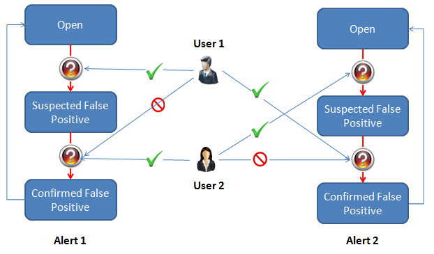
Description of the illustration ''case_man_admin_4eyeprocess.png''
As shown above, User 1 can mark Alert 1 as a Suspected False Positive, and therefore cannot mark it as a Confirmed False Positive. Only another user (User 2 in this case) can do this.
Similarly, if User 2 escalates Alert 2 to a Suspected False Positive, only User 1 can mark it as a Confirmed False Positive.
Below is a screenshot of how a simple 4-Eyes workflow may appear in the Workflow Editor. The three possible States (Open, Suspected False Positive, Confirmed False Positive) and Transitions (Suspect false positive, Confirm false positive and Reopen) are shown in their respective lists:
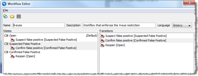
Description of the illustration ''case_man_admin_4eye_workflow_665x256.png''
To enforce the 4-eye rule, the Transitions must be configured as follows:
-
No restrictions are required for the Suspect false positive Transition.
-
Confirm false positive - Add the Suspect false positive Transition to the Blocking Transitions field. This prevents a user applying the Confirm false positive Transition if they made the Suspect false positive Transition.
-
Reopen - Add the Confirm false positive Transition to the Clear Blocking Transitions field. This clears any restrictions on the Confirm false positive Transition being applied to the Alert, for all users.
1.2.6 Configuration Analysis
Configuration Analysis is a part of the EDQ suite of applications. Configuration Analysis can be used to report on the configuration of a project in Director, or on any of the components that make up a project, such as Jobs, Processes and Results Books.
Configuration Analysis can be used to report on the configuration of a component (or set of components), or to compare two components (or sets of components), and report on the differences between them.
The user interface for Configuration Analysis includes:
-
A set of menus and a toolbar, at the top of the screen;
-
Two selection panes at the left of the screen, which are used to select the components to be analyzed;
-
A results area which takes up the remainder of the screen, used for displaying the results of the analysis.
The menus and main toolbar provide the main controls for using Configuration Analysis. All the controls are present on the toolbar and in either the File or Analysis menus. The Help menu provides access to the online help for Configuration Analysis and to the About dialog for the application.
Using the toolbar or corresponding menus, you can:
-
Start a configuration comparison;
-
Start a configuration report;
-
Cancel a comparison or a report;
-
Configure the comparison settings;
-
Configure the report settings;
-
Save results in an HTML format.
The selection panes are used to specify the components for analysis. If a component is selected in just one of the panes, you can run a configuration report for that component.
If one component is selected in each pane, you can compare the configuration of the two components against each other.
When a comparison is performed, changes are expressed relative to the component selected in pane A. For example, suppose that you have compared two processes. If the report states that a processor has been added, then the processor will be absent from the process selected in pane A, and present in the process selected in pane B.
The Result pane displays the results of the most recent comparison or configuration report. The results area is subdivided into multiple panels, and the layout depends on the complexity of the components being analyzed.
The Result pane always contains a component list, which displays the top-level components included in the analysis, and a details pane which contains the details of the report for the currently selected component:
If you select a process in the component list, a processor list will be added to the details pane. This contains a list of all the processors in the selected process.
The component list holds a list of all the components covered by the analysis. If analysis is performed on a single component, such as a process or a set of reference data, there will only be a single entry in this list. If multiple components are covered by the analysis, there will be multiple entries in the list.
The information presented in the results area depends on whether you are browsing comparison results or configuration report results. For report results, each line simply contains the component name and an icon indicating the type of the component (job, process, snapshot and so on).
For comparison results, each line contains the name of the component as seen on both sides of the comparison, and the result of the comparison. The Comparison Filter can be used to filter the items in the list based on the results of the comparison (see Filtering Comparison Results for more details).
For more details, see the comparison results and report results topics, respectively.
The details pane contains a list of the various configurable attributes for the selected component, and their values. When comparing two components, the configuration differences are highlighted using colored backgrounds for the appropriate rows.
Whether you are running comparisons or configuration reports, the results are provided complete with automatically inserted hyperlinks for ease of navigation. The hyperlinks are rendered in blue, underlined text, and can be used to move between the sections of data for a component, or between components.
Each section, such as the 'Options' section, is preceded by a link back to the top of the current page of the report. Subsections are preceded by a link back to the top of the page, and a link to the top of the section.
In addition, links are provided to the previous and next processors in the process.
If you click on a hyperlink in a report, you will build up a browsing history based on your path through the report. This will activate the navigation buttons at the top of the details pane, which can then be used to retrace your path through the report, as required:
The processor list only appears when a process is selected in the component list. The processor list contains a list of all the processors in the selected process. If a comparison is being performed, each row shows the processor as it appears in each version of the process, and the results of comparing those two processors.
For each processor, its name and type are given (for each side of the comparison, if appropriate). It is possible to filter the results by processor name and processor type, if required (see Filtering Comparison Results and Filtering Report Results for more details). In addition, if the process includes grouped processors, the Parent column will be visible. This column shows the group to which the processor belongs.
Navigating from the Processor List to the Canvas
If you have launched Configuration Analysis from within Director, a link is created between the applications. You can use this link to navigate from processors listed in the analysis results back to the location of those processors on the Canvas.
To navigate from the results to the Canvas, right click on the results row which corresponds to the processor you want to investigate.
The options you are offered depend on the type of analysis you have performed and, in the case of comparisons, the results associated with the selected processor:
-
For configuration reports, you are always offered 'View Processor A in Process'. Selecting this option opens the process on the canvas, with the selected processor highlighted. 'View Processor B in Process' is disabled.
-
For configuration comparisons where the processor is present in both versions of the process, both 'View Processor A in Process' and 'View Processor B in Process' are enabled. Selecting 'View Processor A in Process' opens the process selected in selection pane A, with the selected processor highlighted. Selecting 'View Processor B in Process' opens the process selected in selection pane B, with the selected processor highlighted.
-
For configuration comparisons where the processor has been added (that is, it is present in the process selected in selection pane B but not in the process from selection pane A), 'View Processor A in Process' is disabled. Selecting 'View Processor B in Process' opens the process selected in selection pane B, with the selected processor highlighted.
-
For configuration comparisons where the processor has been deleted (that is, it is present in the process selected in selection pane A but not in the process from selection pane B), 'View Processor B in Process' is disabled. Selecting 'View Processor A in Process' opens the process selected in selection pane A, with the selected processor highlighted.
1.2.7 Issue Manager
The Issue Manager application is used to view, assess and manage issues.
You can launch the Issue Manager from either from the EDQ Launchpad, from an Issue notification email, or by clicking on the You have n issue(s) link in the Director Toolbar.
When the Issue Manager is launched, all open issues that are assigned to the logged on user are displayed by default:
The issues displayed can be filtered using the Server, Project and Show drop-down fields, and the Show... check boxes. The Filter menu bar button shows or hides the filtering options.
To open an issue, either right click on it and select Open Issue or double click it. The issue is opened in a separate dialog box.
On this dialog, issues can be reassigned to other users, or marked as "New", "In Progress" or "Complete" in the Status field. It is also possible to open the process the issue originates from by clicking the Related Process link.
Note:
Issues cannot be assigned to users that do not have permission to view the project the issue originates from.1.2.8 Web Service Tester
The Web Service Tester is used to test a running Web Service before any integration work is done.
To open the Web Service Tester, select the Web Service Tester from the Web Services dropdown menu; the service loads automatically once selected.
If started from the Web Service application, the selected Web Service will be displayed by default. If not, then no Web Service is selected.
To test a web service:
-
Select the Project and the Web Service in the Setup area.
-
Click Get Service to retrieve the latest version of the WSDL file. The Web Service inputs are listed in the In area.
-
Enter the available details in the fields and click Send. If the Web Service is running, the results are returned in the Out area.
To run a timing test:
-
Click Timing test. The Timing Test dialog is displayed.
-
Enter the number of times the test is to be performed in the Number of requests field.
-
If required, enter a delay in milliseconds between tests in the Interval (ms) field.
-
Click Run. The Status area shows the progress of the test, and the results when it is complete.
-
If required, click View Chart. The Timing Chart dialog is displayed.
Some Web Services are configured to expect multiple records, i.e. when they were created the Multi Record? option was ticked. A typical example is a Web Service designed to identify matching records from a set of candidates.
For such Web Services, it is possible to add extra records before sending the request. Simply click Add record as many times as is required.
Note:
The Add record button is disabled if the selected Web Service expects a single record.Alternative Integration Methods (JMS)
EDQ also supports integration with its real-time capabilities via JMS (Java Messaging Service). The integration between the real-time providers and consumers must be configured manually.
1.2.9 How To Topics
For How to topics, which provide details of how to perform certain key tasks in EDQ, see "How To" in Oracle Fusion Middleware Using Oracle Enterprise Data Quality.
1.3 Processor Library
Processors available in Oracle Enterprise Data Quality.
1.3.1 Advanced Processors
Advanced processors allow you to perform advanced functions in EDQ, such as defining custom processing using scripting or expressions, or generating warnings from data processing. Advanced processors are intended for use by expert users.
It is also possible to write your own processors and add them into the EDQ palette. See Extending EDQ.
1.3.1.1 Add Message ID
The Add Message ID processor adds a field containing a numeric identifier in to a process. Message IDs identify a packet of data, known as a message, as it passes through an EDQ process.
Add Message ID is used to add a numeric identifier to records. The message ID is unique within a data stream for records in batch processes and records created by real-time processes with single record inputs.
Note that, for a given data stream, this identifier will not be unique in the following circumstances:
-
The Message ID will not be unique for records originating from real-time processes or web services which have multi-record inputs. In this case, the message ID will be the same for all the records originating from a single request.
-
The Message ID will not be unique if records within a stream are split by the process. In this case, the message ID will be the same for all records derived from a single originating record.
The Add Message ID processor presents no summary statistics on its processing.
In the Data view, the added output attribute is shown.
In this example, the message ID has been added to a set of records in a batch process. The process has been run in batch mode, and does not split records, so in this case, the message IDs are all unique:
1.3.1.2 Add User Details
The Add User Details processor adds in to a process details of the authenticated EDQ user calling the Web Service or Job where the process is used.
Add User Details is normally used in applications that use EDQ Web Services for data validation, cleansing or matching. Capturing the details of the authenticated user in the EDQ process is useful for two reasons:
-
To keep a full audit trail of all records processed including details of the user that entered/updated the record
-
So that the process can use the user details, for example to send an email to the authenticated user's address with the results of data processing
For example, where EDQ is used to screen individuals against watchlists, an email may be sent out to the authenticated user of the individual screening service with the result of the matching process, using the email address stored for the user in EDQ (as set up by an administrator in User Configuration). Additional user details, such as organization and phone number, may be added to the audit trail so that complete information on the user submitting the record is retained.
1.3.1.3 Expression
The Expression processor allows you to write an expression which may encompass the logic of a number of other EDQ processors and other functions, using an abbreviated expression language.
Expressions are useful where the required logic of a processor can be expressed most logically and succinctly by writing an expression, rather than by configuring several processors. This is commonly the case when performing mathematical operations, for example.
The Expression processor may take any number of inputs, of any type, with the exception of formal Date attributes.
| Option | Type | Purpose | Default Value |
|---|---|---|---|
| Expression to evaluate | Expression | The required processor logic, in EDQ's expression language. See notes below. | None |
See Expression Notes for detailed notes on EDQ's expression language.
Data Attributes
| Data Attribute | Type | Purpose | Value |
|---|---|---|---|
| ExpressionResult | Added | Stores the result of the expression | An attribute with the result of the expression. The attribute type depends on the expression. See notes above. |
Flags
None
| Execution Mode | Supported |
|---|---|
| Batch | Yes |
| Real-time Monitoring | Yes |
| Real-time Response | Yes |
The Expression processor presents no summary statistics on its processing.
In the Data view, each input attribute is shown with the ExpressionResult attribute to the right.
None
1.3.1.4 Expression Filter
The Expression Filter processor allows you to write an expression using EDQ's expression language, which will be used to pass or fail records and split them into different output filters.
The Expression Filter processor is effectively an advanced form of the Logic Check processor, which provides a GUI to construct the expression. As the Logic Check GUI shows the expression as it is constructed, it is therefore possible to learn how valid expressions are constructed using Logic Check.
Expression Filter is useful where you want to apply a simple test to all input records, and split out records that pass the test from records that fail it.
The Expression Filter processor may take any number of inputs, of any type, with the exception of formal Date attributes.
| Option | Type | Purpose | Default Value |
|---|---|---|---|
| Logic expression | Expression | The required filter logic, in EDQ's expression language. See notes below. | None |
See Expression Notes for detailed notes on EDQ's expression language.
Data Attributes
None
Flags
| Flag | Purpose | Possible Values |
|---|---|---|
| ExpressionFilter | Stores the result of the expression filter test | Y - if the test passed
N - if the test failed |
| Execution Mode | Supported |
|---|---|
| Batch | Yes |
| Real-time Monitoring | Yes |
| Real-time Response | Yes |
The following output filters are available from an Expression Filter processor:
-
True - that is, records that passed the expression filter test
-
False - that is, records that failed the expression filter test
1.3.1.5 Generate Warning
The Generate Warning processor is designed to generate a warning, and/or trigger a process failure, in the event of processing a certain number of records (over a configurable threshold).
Use the Generate Warning processor in conjunction with the notification capabilities in Jobs if you want to be made aware of any warnings when running processes. For example, you might use an audit processor to check for data validity, and you might want to raise a warning if >n records fail the check. You might even want to fail the process to ensure that you don't continue running, if you know the remaining parts of the process need to be rerun in any case.
The Generate Warning processor therefore allows you to set your own definition of what constitutes a 'data error' that you want to see in the Event Log and in any notification emails.
Generate Warning and Intelligent Execution
To avoid generating unnecessary warnings when running the same process repeatedly while designing it, the Generate Warning processor only generates a new warning if its rerun marker is set, or if run in a process or job with intelligent execution turned off.
The rerun marker will always be set if a new set of data is being input to the process, or if the configuration of the processor is changed.
1.3.1.6 Message Handling Script
The Message Handling Script processor allows you to specify your own processor logic using JavaScript or Groovy, entered as an option for the processor.
The Message Handling Script processor is closely related to the Script processor. The main difference between this processor and the Script processor is that the Message Handling Script processor is designed to handle messages, which may contain many records. The Message Handling Script processor is capable of performing operations over all the records in a message, and has access to message level attributes such as the message ID.
Use the message handling script processor to define processing logic that acts across all the records in a message, or that acts selectively on only the first record in the message.
The Message Handling Script processor presents no summary statistics on its processing.
In the Data view, each input attribute is shown with the output attributes to the right.
The following notes are important to consider when writing a script for the Message Handling Script processor.
The Message Handling Script processor takes a message as its unit of work. A message may be composed of multiple records, which are modeled as an array named records within the Message Handling Script processor. Each record in the array has its own set of input attributes and its own output attribute, corresponding to the input1 and output1 attributes of the standard Script processor.
In addition, a pre-defined variable, messageid, contains the unique message ID, and a variable tags, which contains the message level tags.
Each record also has a cancel() function, which suppresses further processing of the record in the process.
Note:
It is possible to specify a function to be called for each record (as opposed to executing the entire script each time), and to change the language of the script.To set a function include the line:
#! function : doit
at the top of the script (where 'doit' is the function name; change this to the function name you are using).
To change the language of the script to groovy rather than Javascript, add the line:
#! language : groovy
The following script iterates across all the records in a message to calculate the sum of the values of the first input attribute for each record (which is assumed to be a number). It then iterates across the records a second time, and sets the value of the output attribute of each record to the sum calculated in the first step:
var sum = 0;
for (var i = 0; i < records.length; i++)
{
  sum += records[i].input1[0];

}

for (var i = 0; i < records.length; i++)
{
  records[i].output1 = sum;

}
The following script computes the sum as before, but all but the first record are suppressed using the cancel() function. This results in a single record - the first - being output per message, with the total of the first input attribute across all records as its output attribute.
var sum = 0;
for (var i = 0; i < records.length; i++)
{
  sum += records[i].input1[0];

}

for (var i = 0; i < records.length; i++)
{
  if (i == 0)

  {

    records[i].output1 = sum;

  }

  else

  {

    records[i].cancel();

  }

}
1.3.1.7 Script
The Script processor allows you to specify your own processor logic for a simple processor using JavaScript or Groovy. The script is entered as an option on the script processor.
Note that it is possible to use a script in a processor that is created in EDQ, so that the script is not easily accessible by the end user of the processor. It is also possible to use script when writing a new processor to add into the processor library - this allows for greater complexity in the script - for example to enable multiple inputs and outputs, options that use Reference Data, and results views.
Use the script processor to define some simple processing logic that cannot be achieved easily using any of the provided processors.
Any number of attributes of any type may be input to a Script processor. The selected input attributes are mapped to a JavaScript array named input1.
| Option | Type | Purpose | Default Value |
|---|---|---|---|
| Result type | Selection (String / Number / Date / String Array / Number Array / Date Array) | Determines the type of the output result of the script.
Note: If you select an Array type, you must instantiate the array in your script. |
String |
| Script | Script | The script defining the processor logic. See note below regarding the use of functions, and changing the script language. | None |
Note:
It is possible to specify a function to be called for each record (as opposed to executing the entire script each time), and to change the language of the scriptTo set a function include the line:
#! function : doit
at the top of the script (where 'doit' is the function name; change this to the function name you are using).
To change the language of the script to groovy rather than Javascript, add the line:
#! language : groovy
The Script processor supports a single output data attribute only. The type of this attribute is determined by the setting of the Result type option.
The single output must be assigned to the script name output1.
Note:
Selecting an Array type for your result type does not automatically instantiate the array. Due to the differences between simple data types and array types, the array must be instantiated by your script. Failure to do this will result in a script execution error when the processor is run. Please see Example 1-3 for more details.| Data attribute | Type | Purpose | Value |
|---|---|---|---|
| ScriptResult | Added | An attribute with the result of the script. | The value is set by the script. |
None
| Execution Mode | Supported |
|---|---|
| Batch | Yes |
| Real-time Monitoring | Yes |
| Real-time Response | Yes |
Note:
When writing a new processor (which may include the use of script), it is possible to make the processor incompatible with Real-time Response execution, by flagging the processor as one which needs to run to completion (for example a processor that filters records based on a percentage calculated across all records that are processed).The Script processor presents no summary statistics on its processing.
In the Data view, each input attribute is shown with the output attributes to the right.
None
Example 1-1 Script to output a unique identifier
The following example script uses an underlying Java function to generate a unique ID.
output1 = java.util.UUID.randomUUID().toString()
In this case, no input attributes are actually used by the script but a dummy attribute must be input to the Script processor to allow it to run.
Result
| ScriptResult |
|---|
| 4d8ed32a-4175-409a-a752-3619cf9fbd5a |
| 8818e732-f56d-4658-bfd9-93ef7ee639bd |
| 4e957a42-6b6c-4669-a7fe-d5c17f1e734f |
| 49a658c1-20db-4d3c-81d8-8cc4aa91016b |
| 1dc94a3c-ec7c-4191-a199-ce1aa4316404 |
| 11d3c22f-77cf-4ccc-bbcf-e78ac2ebd227 |
| dd698c8d-9bfb-40b5-a5bd-2660787233ec |
| b624911b-9d16-4377-8520-4ab546132dfc |
| 7859603f-3348-4bae-ba62-e24daa11c1cd |
| 065fcae7-3a71-4683-931a-cd16c8d45d91 |
| ecdad97d-6dd2-4556-9f47-76cc9a4d74e9 |
| b22b386f-c655-4497-9ee4-a379381201dc |
| 7e7b817d-a752-4b9c-98ca-bfd2c85136fa |
The following example script concatenates all input attributes into a single output value, with each attribute value separated by ||:
var res = '';
for (var i = 0; i < input1.length; i++)
  { if (i > 0) res += '||';
     res += input1[i];
  }
output1 = res;
Result
| Title | Forename | Surname | Name |
|---|---|---|---|
| KAREN LOUSE | MILLER | ||KAREN LOUISE||MILLER | |
| MR | BRIAN MICHAEL | MILES | ||BRIAN MICHAEL||MILES |
| FREDRIK | MISTANDER | ||FREDRIK||MISTANDER | |
| MR | KENNETH | MIDDLEMASS | ||KENNETH||MIDDLEMASS |
| NEIL ALASTAIR | MITCHELL | ||NEIL ALASTAIR||MITCHELL | |
| KOKILA RAMESH | MISTRY | ||KOKILA RAMESH||MISTRY | |
| ANDREW SIMON | MICKLEBURGH | ||ANDREW SIMON||MICKLEBURGH |
Example 1-3 Using an Array Result Type
Unlike simple data types, an array variable must always be instantiated before values can be written to it. Failing to do this will result in an error messages similar to the following:
Script execution failed: TypeError: Cannot set property '0.0' of null to '<value>' ([script]#2)
To instantiate your output array, your script must use the new command to allocate memory for the array, as follows:
var output1 = new Array();
Following this statement, the array will be instantiated and available for writing.
1.3.2 Audit Processors
Audit processors, or checks, check input data using business rules in order to assess whether or not it is fit for its business purpose.
The audit processors used to check data, and the rules used by them, are normally determined from the results of Profiling.
Audit processors categorize each input record as to whether it was valid or invalid according to the check. Invalid records may be handled separately from valid records in downstream processing, using an Output Filter - for example so that you only attempt to clean records that did not pass your check. Some audit processors, such as List Check, have three output filters - valid (the record passed the check), invalid (the record was positively identified as a failure), and unknown (the record was not recognized as either definitely valid, or definitely invalid).
Audit processors implicitly use the business rules that you apply to a given data attribute when profiling. Refer to the following table for the audit processor for each type of business rule that you can apply.
| Type of Rule | Example Business Rule | Audit Processor |
|---|---|---|
| Whether or not the attribute is allowed to contain null values | The CU_NO attribute must not be null | No Data Check |
| The allowed or expected length of the data in the attribute | The CU_ACCOUNT attribute must be between 10-11 characters in length, and must not contain spaces | Length Check |
| The data type consistency in an attribute | There must be no numeric values in the NAME attribute | Data Type Check |
| The validity of values in an attribute | Values in the TITLE attribute must match a list of valid titles | List Check |
| The conformity to a standard character pattern | Values in the TEL_NO attribute must conform to a standard pattern | Pattern Check |
| The conformity to a standard pattern, by regular expression | UK National Insurance Numbers must match a standard regular expression | RegEx Check |
| The validity of specific characters in an attribute | The values in a NAME attribute must not contain characters such as #~@;:/?.>,<%$£!^* | Invalid Character Check |
| Duplication of values in an attribute | There must be no duplicate CU_NO values | Duplicate Check |
| Whether or not the attribute contains any common user entry workarounds for mandatory fields | There must be no values such as 'aaa' in the FORENAME attribute | Suspect Data Check |
| Check one attribute's value against another | The DATE_OF_BIRTH attribute must be before the DATE_OF_DEATH attribute | Cross-attribute Check |
| Check for related data in a reference table | There must be at least one active Contact record for a Customer | Lookup Check |
| Check for data which passes a Logic expression | There is a valid DATE_OF_BIRTH attribute and a valid Postcode and a valid email address | Logic Check |
| Check that data has a specific value, or value range | All male Customers must have a Gender value of 'M' | Value Check |
| Check that data conforms to a set of business rules, defined independently of EDQ. | If the customer is based in England, the post code must be present and must be in a valid format. | Business Rules Check |
In addition to the general-purpose audit processors above, EDQ comes with a number of checks for specific attributes; for example, the Email Check.
Note:
If you cannot create your own check using the general purpose processors provided, you may either write your own check using JavaScript, or you may choose to extend EDQ to add a new processor. See Extending EDQ for more information.1.3.2.1 Business Rules Check
The Business Rules Check processor enables users to check data against a set of business rules, which can be defined and maintained outside of EDQ. Validation errors can be output for each record checked.
The Business Rules Check processor is used to apply potentially complex validation rules to data in a single processor. The business rules can be defined in reference data or in an external file, allowing the rules to be maintained externally to EDQ.
The following tables describe the configuration options:
| Configuration | Description |
|---|---|
| Inputs | The processor accepts:
See Defining Business Rules for information on how to define business rules. |
| Options | Specify the following options:
|
If an Excel file is used to define the business rules, it must be placed in the [Install Path]/oedq_local_home/businessrules directory, where [Install Path] represents the root of the EDQ installation, and must conform to the format specified in the Defining Business Rules topic.
Identifiers are used to map the input attributes of the Business Rules Check processor onto the attribute tags referenced in the business rules document. The mappings between identifiers and attributes are defined on the Identify tab of the Business Rules Check processor dialog.
For each identifier, select the appropriate input attribute from the drop-down on the right.
-
If an identifier which has no mapped input attribute is used in a rule, that rule will be ignored.
-
If an identifier with no mapped input attribute is used in a condition, the condition is assumed to evaluate to
TRUE.
Note:
Unmapped identifiers are treated differently by the Business Rules Check processor, depending on the context.| Configuration | Description |
|---|---|
| Outputs | Describes any data attribute or flag attribute outputs. |
|
Data Attributes |
The following data attributes are output:
|
|
Flags |
The following flags are output:
|
This processor always appears with a re-run marker, indicating that it will be completely re-executed each time the process is run, regardless of whether or not its configuration has changed. This will also mean that processors that are downstream of the processor will need to be rerun. This is because there may be changes made outside of the EDQ application that could lead to different results on subsequent executions.
The following table describes the statistics produced by the profiler:
| Statistic | Description |
|---|---|
| Pass | The number of records which passed the logic check. |
| Fail | The number of records which failed the logic check. |
The following output filters are available from a Logic Check:
-
Records which passed the business rule check
-
Records which failed the business rule check
In this example, the user wants to use an Excel file called contactDetailsCheck.xls to validate some of the contact details in their customer data. This file contains rules which check that:
-
The surname field contains some data;
-
The surname contains only letters;
-
That at least one of Town and County is specified in the address;
-
That the postcode is valid;
-
That the telephone number is valid.
The summary data:
| Pass | Fail |
|---|---|
| 11211 | 1045 |
A drill down on records failing the check shows how those records break the rules, and displays the error codes, severities, and error messages defined as part of the business rules configuration.
1.3.2.1.1 Defining Business Rules
The Business Rules Check processor allows a set of business rules to be defined and maintained outside of EDQ, and applied using a single processor. Rules are defined in terms of attributes, which are independent of any data structure. Attributes have tags such as a1, a2, a3 and so on, and must be mapped to the appropriate fields in the input data when the Business Rules Check processor is configured (see the Business Rules Check topic).
The business rules can be defined:
-
in an Excel file (see Defining business rules in an Excel spreadsheet), or
-
in reference data (see Defining business rules in reference data).
Business rules are made up of three types of component:
-
Checks are small, re-usable pieces of logic. They have a user-defined name, a type of check to be performed, and zero to several options whose meaning varies depending on the type. Checks can be built up to create more complex conditions, or can be used directly in rules. See Defining Checks.
-
Conditions are more complex pieces of logic, which apply checks to attributes, but are not full rules. Using conditions in your business rule configuration is optional, and not always necessary. Conditions can act as a gateway to a rule; if a rule is assigned a condition, the rest of the rule will only be evaluated if the condition passes. Conditions can be built out of checks, or out of other conditions, leading to complex logical structures. See Defining Conditions.
-
Rules specify which checks will be applied to which attributes. A rule has an ID and a label for ease of reference, and also specifies the error code, error message and the severity of the error to be raised if the rule fails. See Defining Rules.
A check has the following characteristics:
-
A name, which is defined by the user and allows the check to be referenced from elsewhere;
-
A check type, which defines the operation that the check will perform, and
-
Up to three options, which provide any additional information that the check operation needs in order to work.
A check does not specify the attribute that it will work against.
The following table describes the supported check types:
| Name | Description | Options |
|---|---|---|
| No Data Check | Used to check that a field is blank. The check will fail if the field contains any data. | None |
| Population Check | Used to check that a field is not blank. The check will fail if the field does not contain any data. | None |
| Character Check | Used to check that data in a field contains only characters from the specified list. | Option 1 = the list of permitted characters (see Note, below), OR
Option 2 = the name of the worksheet containing the permitted characters (for use with Excel-based rules only), OR Option 3 = the name of the reference data containing the permitted characters |
| Invalid Character Check | Used to check that data in a field does not contain any characters from the specified list. | Option 1 = the list of invalid characters (see Note, below), OR
Option 2 = the name of the worksheet containing the invalid characters (for use with Excel-based rules only), OR Option 3 = the name of the reference data containing the invalid characters |
| Min Length Check | Used to specify a minimum length for string data in a field | Option 1 = the minimum length of the data field |
| Max Length Check | Used to specify a maximum length for string data in a field | Option 1 = the maximum length of the data field |
| List Check | Used to check that data in a field contains only values from the specified list. | Option 1 = a single permitted value, OR
Option 2 = the name of the worksheet containing the permitted values (for use with Excel-based rules only), OR Option 3 = the name of the reference data containing the permitted values |
| Invalid List Check | Used to check that data in a field does not contain any values from the specified list. | Option 1 = a single invalid value, OR
Option 2 = the name of the worksheet containing the invalid values (for use with Excel-based rules only), OR Option 3 = the name of the reference data containing the invalid values |
| Regex Check | Used to check that data in a field conforms to a regular expression. | Option 1 = the regular expression, OR
Option 2 = the name of the worksheet containing the regular expression (for use with Excel-based rules only), OR Option 3 = the name of the reference data containing the regular expression |
| Invalid Regex Check | Used to check that data in a field does not conform to a regular expression. | Option 1 = the invalid regular expression, OR
Option 2 = the name of the worksheet containing the invalid regular expression (for use with Excel-based rules only), OR Option 3 = the name of the reference data containing the invalid regular expression |
| Script | Used to specify an external script which will perform processing on the data. | Option 1 = the script code or the name of the script to be executed
Option 2 = the script language. Valid values are 'javascript' or 'groovy'. The language defaults to javascript if no option is specified. |
| Fail | Used to specify a check which will always fail. | None |
Note:
Lists of valid or invalid characters are case sensitive and can include all characters, including alphanumeric characters, whitespace characters and special characters. Where a list is supplied directly in the check, it should be entered as a single string without delimiters or whitespace characters, as these would be interpreted as part of the list itself.Conditions associate checks with attributes. As well as associating a single check with a single attribute, a condition can apply two checks to a single attribute, or a single check to two attributes. It can also be used to aggregate other conditions together to create a more complex condition. Conditions have the following attributes:
-
A name, which is defined by the user and allows the condition to be referenced from elsewhere;
-
A Type field, which specifies the type of the entries in the Condition fields (Checks, Attributes or Conditions);
-
At least one Condition field. Condition fields can contain checks, attributes or conditions, as specified by the Type;
-
An 'Attribute or Check' field, whose content depends on the value of the Type. If the Type is 'Checks', this field contains the attribute to which the checks will be applied. If the Type is 'Attributes', this field contains the check that will be applied to the attributes. If the type is 'Conditions', this field is not used.
-
An Operator field, which can contain one of the logical operators AND, OR and NOT. If this field is set to AND, and a value is set in more than one Condition field, then both the conditions must evaluate to true for the condition as a whole to return true. If set to OR, then only one condition from the set must return true for the whole condition to evaluate To true. If set to NOT, the condition evaluates to the opposite of the expression specified in the first Condition field. If this field is NULL, its meaning is assumed to be 'AND'. The operators AND and OR have no meaning unless at least two conditions fields are set.
The following table summarizes the behavior when two condition fields, named Condition1 and Condition2, are in use:
| If Type is set to... | Then Condition1 and Condition2 contain... | And Attribute or Check contains... | If Condition1 and Condition2 are set, then... | The AND operator will cause the condition to return... | The OR operator will cause the condition to return... |
|---|---|---|---|---|---|
| Checks | A check or checks | An attribute | The two checks will both be applied to the attribute. | TRUE if and only if both conditions return TRUE for the attribute | TRUE if at least one of the conditions returns TRUE for the attribute |
| Attributes |
An attribute or attributes |
A check |
The check will be applied to both attributes. | TRUE if and only if the condition returns TRUE for both attributes | TRUE if the condition returns TRUE for at least one of the attributes |
| Conditions |
Conditions |
Nothing |
Both conditions will be evaluated. | TRUE if and only if both conditions return TRUE | TRUE if at least one of the conditions returns TRUE |
It will readily be seen that by combining checks with different attributes and operators, and aggregating the resulting conditions together to form more complex conditions, complex logical checks can be built up.
Rules are the top-level entities in the business rules check. They bring together checks and conditions, specify which attributes the checks should be applied to, and specify the error code and error message that should be raised if the rule fails. In addition, the severity of the error can be specified at this level.
Rules have the following fields:
-
The Rule ID is a numeric identifier for the rule;
-
The Rule Label is a human-readable name for the rule;
-
The Disable field can be set to 'Yes' to remove the rule from processing without deleting it;
-
The Apply to Attribute field specifies the attribute to which the checks should be applied;
-
The Condition field specifies a condition that should be evaluated before the rule is applied. The rule will not be applied if the condition is not met.
-
The Error Code specifies the error code that will be returned if the rule fails. Error codes are defined entirely at the user's discretion and can be in any format.
-
The Error Message is a user-defined message that will be returned if the rule fails.
-
The Error Severity specifies an indication of the severity of the rule failing. Error severities are defined entirely at the user's discretion and can be in any format.
-
Check 1 specifies the first check to be applied to the attribute;
-
Check 2 specifies the second check to be applied to the attribute.
If two checks are specified, then the rule only passes if the attribute passes both checks. That is, the result is the logical AND of both checks.
Note:
Conditions can be applied to rules in order to ensure a complex set of conditions is not true. The logic describing the invalid configuration is specified using conditions. Then, a very simple rule can be created which is controlled by the condition and has Check 1 set to 'Fail'. When a rule is configured in this way, the condition will be evaluated for each row analyzed, and, if the condition is met, the rule will always fail.Defining business rules in an Excel spreadsheet
If you want to use an Excel Spreadsheet to define your business rules, it must conform to the following rules:
-
It must be placed in the
[Install Path]/oedq_local_home/businessrulesdirectory, where[Install Path]represents the root of your EDQ installation. -
The rules, conditions and checks must be defined on three separate worksheets, named Rules, Conditions and Checks, respectively.
-
You may supply further worksheets in the same Excel file to contain additional data, for use in list checks and so on.
-
The Rules worksheet should contain columns named as follows:
-
Rule ID
-
Rule Label
-
Disable
-
Apply to Attribute
-
Condition
-
Error Code
-
Error Severity
-
Error Message
-
Check 1
-
Check 2
-
-
The Conditions worksheet should contain columns named as follows:
-
Condition Name
-
Attribute or Check
-
Type
-
Operator
-
Condition1
-
Condition2 ... ConditionN
-
-
The Checks worksheet should contain columns named as follows:
-
Check Name
-
Check Type
-
Option 1
-
Option 2
-
Option 3
-
Defining business rules in reference data
If you want to use reference data to contain your business rules, it must conform to the following rules:
-
Three separate sets of reference data (or two sets, if you are not using conditions) must be available, specifying the rules, conditions and checks, respectively.
-
The structure of the reference data must be the same as that described for the Excel spreadsheets, above.
1.3.2.2 Cross-attribute Check
The Cross-attribute Check processor allows you to compare the values in two attributes in order to check the consistent application of a business rule.
Note that you can only compare attributes of the same Data Type; that is, a String attribute must be compared with another String attribute, a DATE with another DATE, and a Number with another Number.
Use Cross-attribute Check to check that the data for two related attributes is correct. For example, you may want to check that Date_Of_Death values are later dates than Date_Of_Birth values.
The following table describes the configuration options:
| Configuration | Description |
|---|---|
| Inputs | Specify two attributes that you want to compare. The attributes must be of the same data type. |
| Options | Specify the following options:
|
| Outputs | Describes any data attribute or flag attribute outputs. |
|
Data Attributes |
None. |
|
Flags |
The following flag is output:
|
The following table describes the statistics produced by the profiler:
| Statistic | Description |
|---|---|
| Records passing comparison | The number of records that passed the comparison. |
| Records failing comparison | The number of records that failed the comparison. |
| Records with null value(s) | The number of records where either, or both, values being compared were null. |
The following output filters are available from a Cross-attribute Check:
-
Pass; that is, records where the comparison passed
-
Fail; that is, records where the comparison failed
-
Null comparison; that is, records with a null value in either or both attributes checked
In this example, two attributes are compared: DT_ACC_OPEN and DT_PURCHASED, to see how many have repeated data:
| Records Passing Comparison | Records Failing Comparison | Records with Null Value(s) |
|---|---|---|
| 996 | 3 | 1 |
You can drill down on the Records Passing Comparison:
| DT_ACC_OPEN | DT_PURCHASED | CrossAttributeCheck |
|---|---|---|
| 03/01/2000 | 03/01/2000 | Y |
| 06/01/2000 | 06/01/2000 | Y |
| 10/01/2000 | 10/01/2000 | Y |
| 14/01/2000 | 14/01/2000 | Y |
1.3.2.3 Data Type Check
The Data Type Check processor checks that the values in a String attribute conform to a consistent data type, and categorizes as invalid any records with values that are not of the expected data type.
Note that Number and Date attributes are by definition 100% consistent with regard to their data type, and so cannot be checked.
The Data Type Check is a useful way of quickly finding values that have been entered into the wrong fields in a user application - typically numbers or dates that have been entered into fields that expect text values only.
Note that it is possible to 'expect' dates or numbers in a String attribute, and categorize as invalid any values that are not of the expected type. This is provided because dates and numbers are not always held in attributes with a controlled data type that can be read from the schema of the data source.
The following table describes the configuration options:
| Configuration | Description |
|---|---|
| Inputs | Specify a single String attribute that you want to check for data type consistency. |
| Options | Specify the following options:
|
| Outputs | Describes any data attribute or flag attribute outputs. |
|
Data Attributes |
None. |
|
Flags |
The following flag is output:
|
The following table describes the statistics produced by the profiler:
The Date Formats Reference Data used by the Data Type Check must conform to the standard Java 1.6.0 or later SimpleDateFormat API.
| Statistic | Description |
|---|---|
| Valid | Records with data of the expected data type in the input attribute. |
| Invalid | Records with data not of the expected data type in the input attribute. |
Clicking on the Additional Information button will show the above statistics as percentages of the total number of records analyzed.
The Data Type Check produces the following output filters:
-
Valid records
-
Invalid records
In this example, the Data Type Check is used to check that all values for a NAME attribute are in textual format.In this case, null values are treated as invalid.
| Valid | Invalid |
|---|---|
| 2008 | 3 |
In this case, a date value that was entered into the wrong field, and two Null Name values were found.
1.3.2.4 Duplicate Check
The Duplicate Check processor provides a simple way of checking for duplicate values across either one or many attributes.
Use the Duplicate Check to identify any duplicate values that may cause a problem for a data migration (for example, in key attributes), or as an initial check for duplicate records in the data.
The following table describes the configuration options:
| Configuration | Description |
|---|---|
| Inputs | Specify all attributes that you want to consider in the duplicate check. Records will be identified as duplicates if they are the same in all input attributes. |
| Options | Specify the following options:
|
| Outputs | Describes any data attribute or flag attribute outputs. |
|
Data Attributes |
None. |
|
Flags |
The following flag is output:
|
The Duplicate Check assesses duplication across a batch of records. It must therefore run to completion before its results are available, and is not suitable for a process that requires a real time response.
When executed against a batch of transactions from a real time data source, it will finish its processing when the commit point (transaction or time limit) configured on the Read Processor is reached. The statistics returned will indicate the number of duplicates in the batch of transactions only.
The following table describes the statistics produced by the profiler:
| Statistic | Description |
|---|---|
| Duplicated | The records that were duplicated in the input attributes. Drill down to see each distinct value, and the number of times it occurred. Drill down again to see the records. |
| Not duplicated | The records that were not duplicate in the input attributes. |
The following output filters are available from a Duplicate Check:
-
Duplicate records
-
Non-duplicate records
In this example, the Duplicate Check processor is used to look for duplicate company names in a BUSINESS attribute:
| Duplicated | Not duplicated |
|---|---|
| 41 | 1970 |
You can drill down on duplicated values:
| Business | Count |
|---|---|
| Test | 3 |
| Zircom | 2 |
| Darwins | 2 |
| Tamlite Group | 2 |
| BSA Guns (UK) Limited | 2 |
| Permanent Pest Control | 2 |
| Gemini Visuals | 2 |
| Northern Water Utilities | 2 |
| Attitude Flooring | 2 |
| N S News & Confectionery | 2 |
| Send Group | 2 |
| Press Patterns | 2 |
1.3.2.5 Email Check
The Email Check processor checks for Email Addresses in an attribute, and validates them syntactically; that is, that the address conforms to a correct pattern for Email Addresses.
Note that Email Check uses a reference list of regular expressions to check for valid email addresses. You may change the rules used by the Email Check by modifying the list of regular expressions used for the check.
Use the Email Check processor to validate that email addresses have been entered correctly.
Note:
The Regular Expression used to validate email addresses is not foolproof. It will pass as valid email addresses containing a "." immediately after an "'@" symbol. It is recommended that an additional check be run on the Valid output of this processor to check for instances of such incorrectly formatted email addresses.The following table describes the configuration options:
| Configuration | Description |
|---|---|
| Inputs | Specify a single attribute that you want to check for valid email addresses. |
| Options | Specify the following options:
|
| Outputs | Describes any data attribute or flag attribute outputs. |
|
Data Attributes |
None. |
|
Flags |
The following flag is output:
|
The following table describes the statistics produced by the profiler:
| Statistic | Description |
|---|---|
| Valid records | Records with an email address in a valid pattern in the checked attribute. |
| Invalid records | Records where the data in the checked attribute was not in a valid email address pattern. |
The following output filters are available from an Email Check:
-
Valid records
-
Invalid records
In this example, Email Check is used to check data in an EMAIL attribute:
| Valid Records | Invalid Records |
|---|---|
| 1978 | 2 |
You can drill down on valid or invalid values.
Invalid values:
| [email protected] |
| shirley.bayer@angela's.com |
1.3.2.6 Invalid Character Check
The Invalid Character Check processor provides a quick and easy way to find values that contain odd characters.
Use the Invalid Character Check to check for unusual characters. This is particularly useful when analyzing free text fields, which may have 'data cheats' in them, where data entry users have worked round mandatory fields by entering dummy characters such as #. The Invalid Character Check is also useful for finding typos.
If the invalid characters do not signify anything, they can simply be removed by adding a Denoise processor.
The following table describes the configuration options:
| Configuration | Description |
|---|---|
| Inputs | Specify a single attribute to analyze for invalid characters. |
| Options | Specify the following options:
|
| Outputs | Describes any data attribute or flag attribute outputs. |
|
Data Attributes |
None. |
|
Flags |
The following flag is output:
|
The following table describes the statistics produced by the profiler:
| Statistic | Description |
|---|---|
| Valid records | The records that were categorized as valid by the Invalid Character Check. |
| Invalid records | The records that were categorized as invalid by the Invalid Character Check. |
The following output filters are available from a Invalid Character Check:
-
Valid records
-
Invalid records
In this example, a NAME attribute is checked for invalid characters such as ()#%^*$£"!A number of records are found containing the # character.
| Valid | Invalid |
|---|---|
| 1988 | 13 |
You can drill down on invalid values:
| Name |
|---|
| # MCAULEY |
| # RAE |
| # WILLIAM |
| # SWAN |
| # HAWKES |
| # BARKER |
| # PALMER |
| # SNOWDON |
| # DOONAN |
| # MCCLEMENTS |
| # SHIELDS |
| # SEADEN |
1.3.2.7 Length Check
The Length Check processor provides a quick and easy way for checking an attribute for values of the appropriate length.
The Length Check can check either, or both, of the following:
-
The total length in characters (including whitespace and control characters)
-
The number of words
You can choose the way 'words' are counted using options on the Length Check. By default, words are separated by spaces. For example, the word count of 'Oracle Limited' is 2.
Use the Length Check to ensure that the data within the attribute will meet either its technical or business purpose. For example, if migrating an attribute's data to a shorter attribute in a target system, you may choose to truncate the data, and then check that it conforms to the character length restrictions of the target field before migrating. Alternatively, there may be a business reason why a value should not be over a set number of characters, or words. For example, you might want to check a Surname attribute for all values over 2 distinct words in length, as this might indicate misuse of the attribute - for example to store a Company Name value.
The following table describes the configuration options:
| Configuration | Description |
|---|---|
| Inputs | Specify a single attribute that you want to check for values that are too short or too long. |
| Options | Specify the following options:
|
| Outputs | Describes any data attribute or flag attribute outputs. |
|
Data Attributes |
None. |
|
Flags |
The following flag is output:
|
The following table describes the statistics produced by the profiler:
| Statistic | Description |
|---|---|
| Both counts good | The number of records with valid character and word counts. |
| Bad char, good word count | The number of records with an invalid character count, but a valid word count. |
| Good char, bad word count | The number of records with a valid character count, but an invalid word count. |
| Both counts bad | The number of records with invalid character and word counts. |
Click on the Additional Data button to see the above statistics as percentages of the number of records analyzed.
The following output filters are available from a Length Check:
-
Valid (records where both counts were valid)
-
Invalid (records where both counts were invalid)
-
Invalid character count (records with an invalid character count, but a valid word count)
-
Invalid word count (records with an invalid word count, but a valid character count)
In this example, Length Check is used to check the length of an Account Number attribute (CU_ACCOUNT) for any values with a character count not in the range 10-11, and any values that do not consist of a single word:
| Both counts good | Bad char, good word counts | Good char, bad word counts | Both counts bad |
|---|---|---|---|
| 2002 | 4 | 0 | 4 |
You can drill down on a bad character, good word lengths count.
Note that the CU_ACCOUNT attribute for the above records is too short.
| CU_ACCOUNT | CU_NUMBER |
|---|---|
| 97-19601- | 10944 |
| 02-999-ZZ | 99999 |
| 00-000-ZZ | |
| 00-0-XX | 0 |
1.3.2.8 List Check
The List Check processor checks the data in an attribute against reference lists of valid and invalid values for the attribute.
The List Check allows case sensitive or insensitive matching, and can match the reference lists in one of a number of different ways:
-
Contains (the value must contain a matching list entry)
-
Whole value (the value must match the list exactly)
-
Starts with (the value must begin with a matching list entry)
-
Ends with (the value must end with a matching list entry)
-
Delimiter match (match the list after splitting the data using the specified delimiters)
Note:
The List Check processor does not support the use of External Reference Data for the valid or invalid values. Attempting to do so will result in an error message during processing.The List Check is an important processor, used in auditing to find valid and invalid values in a data attribute. Use the results of the Frequency Profiler or Phrase Profiler to create lists of valid and invalid values, and use them in a List Check to audit the data against the lists on an ongoing basis.
List Check allows the use of up to two reference lists - a list of Valid values for the attribute, and a list of Invalid values.
You may choose only to use one of these two lists. For example, if you discover from profiling that there are many different valid values for an attribute, you may want only to check the attribute for invalid values, and consider the non-matching values as either Valid, or Unknown - for example simply to look for suspect words such as 'Test' in a Surname attribute.
If, however, the attribute has a small number of valid values, you may want simply to check the data against a list of valid values, and consider the non-matching values as Invalid, or Unknown - for example to check Title values against a small set of valid titles.
Finally, you can use both lists, and recognize both valid and invalid values, with values that do not match either list categorized as Unknown.
The following table describes the configuration options:
| Configuration | Description |
|---|---|
| Inputs | Specify a single attribute that you want to check based on lists of valid or invalid values (or both). |
| Options | Specify the following valid value options:
Specify the following invalid value options:
Specify the following match options:
|
| Outputs | Describes any data attribute or flag attribute outputs. |
|
Data Attributes |
None. |
|
Flags |
The following flags are output:
|
The following table describes the statistics produced by the profiler:
| Statistic | Description |
|---|---|
| Valid records | The records that were categorized as Valid by the List Check. |
| Unknown records | The records that were categorized as Unknown by the List Check. |
| Invalid records | The records that were categorized as Invalid by the List Check. |
Drilling down on any of the above statistics reveals a count of the distinct values that were found to be Valid, Unknown or Invalid. You can then drill down again to see the records themselves.
The following output filters are available from a List Check:
-
Valid records
-
Unknown records
-
Invalid records
In this example, the List Check is used to check the values in a Business attribute using lists of valid and invalid Business values collated from Frequency Profiling.
Note that values that do not match either list are categorized as Unknowns.
A summary view:
| Valid Records | Unknown Records | Invalid Records |
|---|---|---|
| 1665 | 332 | 4 |
A drill down on unknown records:
| Value | Count | % |
|---|---|---|
| 331 | 16.5 | |
| Fields | 1 | <0.1 |
A drill down on invalid records:
| Value | Count | % |
|---|---|---|
| Test | 3 | 0.1 |
| Test Ltd | 1 | <0.1 |
1.3.2.9 Logic Check
The Logic Check processor enables users to perform a logic check, using multiple criteria to route or filter records.
The Logic Check processor is normally used as a way to filter records to a required set. For example, if all records are passed through a number of checks, it may be useful to add a Logic Check at the end to select which records are considered as overall passes and fails, using the Flag attributes added by other audit processors.
Logic Check may also be used to filter down records to a specific set where the data matches a number of criteria across a number of attributes.
The following table describes the configuration options:
| Configuration | Description |
|---|---|
| Inputs | Specify any number of attributes of any type (except arrays). |
| Options | Specify the following valid value options:
Note that the options specified drive the construction of an expression that is used to filter records. It is also possible to edit the expression directly, once you have mastered how the expressions are written. The expressions may also be used in the Expression Filter custom processor. |
| Outputs | Describes any data attribute or flag attribute outputs. |
|
Data Attributes |
None. |
|
Flags |
The following flags are output:
|
The following table describes the statistics produced by the profiler:
| Statistic | Description |
|---|---|
| Records Passing Check | The number of records which pass the logic check |
| Records Failing Check | The number of records which fail the logic check |
The following output filters are available from a Logic Check:
-
Records with data in the checked attributes
-
Records without data in the checked attributes
For example, the user wants to filter the records which have all of the following attributes populated: NAME, ADDRESS1, POSTCODE, EMAIL. These attributes are profiled in the Quickstats profiler first to generate the Populated flags.
A summary view:
| Records Passing Check | Records Failing Check |
|---|---|
| 859 | 141 |
You can drill down on the records passing check, or records failing check.
1.3.2.10 Lookup Check
The Lookup Check processor allows you to check for records in a set of Reference Data that are related to those that you are currently working with, for example, data from another table in a relational database, or related data in a separate system.
Lookup Check uses an exact match (using one or more key attributes) to match records in the Reference Data.
Use Lookup Check when you want to check how many related records for each of your working records exist in a Reference Data table. The Check can fail any records that have either too many, or too few, related records, according to configurable options.
For example, you may want to check that there is at least one Address record for each of your Customer records.
The following table describes the configuration options:
| Configuration | Description |
|---|---|
| Inputs | Specify the attributes that you want to use to lookup against the Reference Data. These should correspond to the attribute(s) that compose the lookup column(s) of the Reference Data. |
| Options | Specify the following valid value options:
|
| Outputs | Describes any data attribute or flag attribute outputs. |
|
Data Attributes |
None. |
|
Flags |
The following flags are output:
|
When looking up external data (that is not staged), the appropriate level of performance of the lookup will depend upon there being appropriate indexes on the lookup columns for the selected Reference Data. Also, if looking up external reference data, the Lookup Check processor will always appear with a re-run marker, indicating that it will be completely re-executed each time the process is run, regardless of whether or not the actual processor configuration has changed. This will also mean that processors that are downstream of the Lookup Check processor will need to be rerun. This is because EDQ cannot detect whether or not the external reference data has changed, and therefore has to assume that it has changed (since external lookups are usually used for dynamically changing reference data), and so re-executes the lookup in order to ensure the consistency of dependent results.
The following table describes the statistics produced by the profiler:
| Statistic | Description |
|---|---|
| Valid records | The number of records from the working data with an acceptable number of related records in the Reference Data, according to the configured options. |
| Invalid records | The number of records from the working data with an unacceptable number of related records in the Reference Data, according to the configured options. |
The following output filters are available:
-
Valid records
-
Invalid records
In this example, a Lookup Check is performed to check that at least one order (record in the Workorder table) exists for each Customer record. All Customers without any orders may then be tagged as 'Prospects' and not included in the active Customer statistics:
A summary view:
| Valid Records | Invalid Records |
|---|---|
| 1718 | 292 |
A drill down on invalid records:
| CU_NO | CU_NO.count.1 |
|---|---|
| 13810 | 0 |
| 13833 | 0 |
| 13840 | 0 |
| 13841 | 0 |
| 13865 | 0 |
| 13877 | 0 |
| 13938 | 0 |
| 13950 | 0 |
| 13952 | 0 |
| 13966 | 0 |
| 13971 | 0 |
| 13977 | 0 |
| 14001 | 0 |
1.3.2.11 No Data Check
The No Data Check processor provides a simple way of checking whether or not there is any meaningful data in an attribute, or across a number of attributes.
The No Data Check checks not only for null values, but also for empty Strings, and values consisting entirely of spaces or non-printing characters - though only null values will exist if the data has already undergone No Data Handling in the snapshot.
If a record has any data other than white space in any of the attributes analyzed, it is categorized as containing data. Otherwise, if all attributes analyzed contain No Data, it is categorized as containing no data.
Use the No Data Check processor to check for complete and incomplete values in an attribute, or across a number of attributes. For example, you may want to check for all records that have a missing Gender value, and add it where possible using the data available, perhaps by mapping from a Title attribute. Or, you may want to isolate all records that have no data at all in a number of Name or Address fields.
The following table describes the configuration options:
| Configuration | Description |
|---|---|
| Inputs | Specify any number of attributes that you want to check for completeness. |
| Options | Specify the following valid value options:
|
| Outputs | Describes any data attribute or flag attribute outputs. |
|
Data Attributes |
None. |
|
Flags |
The following flag is output:
|
The following table describes the statistics produced by the profiler:
| Statistic | Description |
|---|---|
| Without Data | The number of records without data in the checked attributes. |
| With Data | The number of records with data in the checked attributes. |
The following output filters are available:
-
Records with data in the checked attributes
-
Records without data in the checked attributes
In this example, the No Data Check is used to find records without an email address (in an EMAIL attribute):
A summary view:
| Without Data | With Data |
|---|---|
| 91 | 1919 |
A drill down on Without Data:
| CU_NO | |
|---|---|
| 14057 | |
| 14072 | |
| 14307 | |
| 14515 | |
| 99999 | |
| 14978 | |
| 12586 | |
| 10087 | |
| 10090 | |
| 13899 | |
| 10187 | |
| 15164 |
1.3.2.12 Pattern Check
The Pattern Check processor checks the pattern of data in an attribute against reference lists of valid and invalid patterns.
Use the Pattern Check processor to ensure that the data in an attribute conforms to one of the valid patterns for that attribute. Data may need to conform to a set of valid patterns for either technical or business reasons. For example, when migrating data, the target system may require that all data for a given attribute consists of numeric characters only, and with minimum and maximum length restrictions. Alternatively, for business reasons, it may be that you want to tag as invalid records that have bad data, or data in the wrong attributes, for example, numeric values in Name fields, malformed product codes etc.
You can create the lists of valid and invalid patterns from the data itself using the Patterns Profiler.
Pattern Check allows the use of up to two reference lists - a list of Valid patterns for the attribute, and a list of Invalid patterns.
You may choose only to use one of these two lists. For example, if you discover from profiling that there are many different valid patterns for an attribute, you may want only to check the attribute for invalid patterns, and consider the non-matching values as either Valid, or Unknown.
If, however, the attribute has a small number of valid patterns, you may want simply to check the data against a list of valid patterns, and consider the non-matching values as Invalid, or Unknown.
Finally, you can use both lists, and recognize both valid and invalid patterns, with values that do not match either list categorized as Unknown.
The following table describes the configuration options:
| Configuration | Description |
|---|---|
| Inputs | Specify a single attribute that you want to check for valid or invalid patterns (or both). |
| Options | Specify the following valid value options:
Specify the following valid pattern options:
Specify the following valid pattern options:
|
| Outputs | Describes any data attribute or flag attribute outputs. |
|
Data Attributes |
None. |
|
Flags |
The following flags are output:
|
The following table describes the statistics produced by the profiler:
| Statistic | Description |
|---|---|
| Valid records | The records that were categorized as Valid by the Pattern Check. |
| Unknown records | The records that were categorized as Unknown by the Pattern Check. |
| Invalid records | The records that were categorized as Invalid by the Pattern Check. |
Drilling down on any of the above statistics reveals a count of the distinct patterns that were found to be Valid, Unknown or Invalid. You can then drill down again to see the records themselves.
The following output filters are available:
-
Valid records
-
Unknown records
-
Invalid records
In this example, Pattern Check is used to verify values in an Account Number attribute (CU_ACCOUNT) using lists of valid and invalid patterns collated from Patterns Profiling.
Values that did not match either list of pattens were categorized as Unknown.
A summary view:
| Valid Records | Unknown Records | Invalid Records |
|---|---|---|
| 1991 | 1 | 9 |
A drill down on invalid records:
| Value | Count | % |
|---|---|---|
| aa-NNNNN-aa | 4 | 0.2 |
| NN-NNN-aa | 2 | <0.1 |
| NN-NNNNN-Na | 1 | <0.1 |
| NN-NNNNN- | 1 | <0.1 |
| NN-N-aa | 1 | <0.1 |
1.3.2.13 RegEx Check
The RegEx Check processor checks the data in an attribute against reference lists of valid and invalid regular expressions for the attribute.
The case-sensitivity and matching technique (Whole Value / Contains / Starts With / Ends With) of the check can be controlled.
The RegEx Check processor is a powerful tool, allowing you to validate data according to its exact content, using the position of data, partial and exact values, and wild cards.
The RegEx Check is useful in order to check any data that should be in a consistent structure, for example, UK National Insurance Numbers.
Regular expressions are a standard technique for expressing patterns and manipulating Strings that is very powerful once mastered.
Tutorials and reference material about regular expressions are available on the Internet, and in books, including: Mastering Regular Expressions by Jeffrey E. F. Friedl published by O'Reilly UK; ISBN: 0-596-00289-0.
There are also software packages available to help you master regular expressions, such as RegExBuddy, and online libraries of useful regular expressions, such as RegExLib.
The following are some examples of regular expressions that could check data:
| Regular Expression | Pattern Meaning |
|---|---|
| ^\d{5}$ | 5 integer US zip code. |
| ([A-Z]{1,2}[0-9]{1,2}|[A-Z]{3}|[A-Z]{1,2}[0-9][A-Z])( |-)[0-9][A-Z]{2} | Valid UK Postcode. |
| ^[A-CEGHJ-PR-TW-Z]{1}[A-CEGHJ-NPR-TW-Z]{1}[0-9]{6}[A-DFM]{0,1}$ | Valid UK National Insurance number. |
| ^([a-zA-Z0-9_\-\.]+)@([a-zA-Z0-9_\-\.]+)\.([a-zA-Z]{2,5})$ | Valid email address. |
The following table describes the configuration options:
| Configuration | Description |
|---|---|
| Inputs | Specify a single attribute that you want to check based on lists of valid and invalid regular expressions (or both). |
| Options | Specify the following valid pattern options:
Specify the following invalid pattern options:
Specify the following match options:
|
| Outputs | Describes any data attribute or flag attribute outputs. |
|
Data Attributes |
None. |
|
Flags |
The following flags are output:
|
The following table describes the statistics produced by the profiler:
| Statistic | Description |
|---|---|
| Valid records | The records that were categorized as Valid by the RegEx Check. |
| Unknown records | The records that were categorized as Unknown by the RegEx Check. |
| Invalid records | The records that were categorized as Invalid by the RegEx Check. |
Drilling down on any of the above statistics reveals a count of the distinct patterns that were found to be Valid, Unknown or Invalid. You can then drill down again to see the records themselves.
The following output filters are available:
-
Valid records
-
Unknown records
-
Invalid records
In this example, a RegEx Check is used to check the format of an Account Number attribute (CU_ACCOUNT), using a Whole Value match against the following regular expression:
^([0-9]{2})(-)([0-9]{4,5})(-)([a-zA-Z]{2})
This regular expression dictates that values must start with exactly 2 digits, following by a hyphen, followed by either 4 or 5 digits, followed by another hyphen, followed by two letters.
A summary view:
| Valid Records | Unknown Records | Invalid Records |
|---|---|---|
| 1997 | 0 | 14 |
A drill down on invalid records:
| Value | Count | % |
|---|---|---|
| 4 | 0.2 | |
| OO-24077-SH | 1 | <0.1 |
| OO-24282-LR | 1 | <0.1 |
| OO-24276-LR | 1 | <0.1 |
| 0975t3487263 | 1 | <0.1 |
| OI-25057-JD | 1 | <0.1 |
| 97-19671-5H | 1 | <0.1 |
| 97-19601- | 1 | <0.1 |
| 02-999-ZZ | 1 | <0.1 |
| 00-0-XX | 1 | <0.1 |
1.3.2.14 Suspect Data Check
The Suspect Data Check processor checks an attribute value for a variety of common data entry 'cheats', such as entering 'aaa' in a name field.
Specifically, it can check for any or all of the following:
-
Repeating alphabetic characters (for example, 'aaa')
-
Repeating numeric characters (for example, '111')
-
Repeating non-alphanumeric characters (for example, '>>>')
-
Repeating patterns (for example, 'abcabc')
-
Minimum character length (for example, for short values such as 'x')
Use the Suspect Data Check to check for common user ruses which result in suspect data in compulsory columns.
Where an empty value cannot be entered at the point of data entry, the user may enter a single character - for example a space, a full stop, or a random single character - to get past that point.
Alternatively, a single but repeating character may be entered - for example '9999' - or perhaps a repeating pattern of characters - for example 'asdasd'.
Note that this may not be the fault of the user, but of the business process and/or supporting applications. The user may not know or have available the complete set of data that the data entry application is requesting, but is required to enter the data into the system.
The following table describes the configuration options:
| Configuration | Description |
|---|---|
| Inputs | Specify a single attribute that you want to check for suspect data entries. |
| Options | Specify the following repeating alphabetic character options:
Specify the following repeating numeric character options:
Specify the following repeating non-alphanumeric character options:
Specify the following repeating patterns options:
Specify the following minimum length options:
|
| Outputs | Describes any data attribute or flag attribute outputs. |
|
Data Attributes |
None. |
|
Flags |
The following flags are output:
|
The following table describes the statistics produced by the profiler:
| Statistic | Description |
|---|---|
| Suspect records | Records that were identified as having a suspect value in the attribute checked.
Drill down to see a breakdown of the suspects by the check that identified them. Drill down again to see the records. |
| Valid records | Records that did not have a suspect value in the attribute checked. |
| Null records | Records with a null value in the attribute checked. |
The following output filters are available:
-
Valid records
-
Suspect records
-
Records that were null in the attribute checked
In this example, the Suspect Data Check is used to check a NAME attribute for suspect data entries.
A summary view:
| Alpha repeats | Numeric repeats | Non-alpha repeats | Pattern repeats | Short values |
|---|---|---|---|---|
| 1 | 1 | 1 | 0 | 0 |
A drill down on Alpha repeats:
| NAME | CU_NUM |
|---|---|
| aaaaaaaaa | 87581 |
1.3.2.15 Value Check
The Value Check processor compares the data in an attribute against a single value.
There are a number of options for performing the comparison:
-
Equals
-
Greater than or equal to
-
Greater than
-
Less than or equal to
-
Less than
Use Value Check as a simple way of filtering records according to the value of a single attribute. This might be to concentrate analysis on an area of interest, or to check values against a threshold value.
The following table describes the configuration options:
| Configuration | Description |
|---|---|
| Inputs | Specify one attribute only (any type). |
| Options | Specify the following options:
|
| Outputs | Describes any data attribute or flag attribute outputs. |
|
Data Attributes |
None. |
|
Flags |
The following flags are output:
|
The following table describes the statistics produced by the profiler:
| Statistic | Description |
|---|---|
| Valid records | Records that passed the value check. |
| Invalid records | Records that failed the value check. |
| Null records | Null records (if the option was used to classify these separately). |
The following output filters are available:
-
Valid records
-
Invalid records
-
Null records
In this example, records are filtered by a Gender attribute, using a value check of 'is equal to M':
A summary view:
| Valid Records | Invalid Records | Null Records |
|---|---|---|
| 819 | 1034 | 148 |
A drill down on valid records:
| GENDER | CU_NUM |
|---|---|
| M | 13815 |
| M | 13841 |
| M | 15531 |
| M | 13870 |
| M | 13913 |
| M | 15912 |
| M | 13941 |
| M | 13950 |
1.3.3 GNR Processors
GNR, or Global Name Recognition, is a suite of APIs produced by the IBM Corporation.
Oracle have integrated with many of these APIs in order to provide analysis, parsing and matching of names based on GNR's extensive dictionaries of linguistic name variants.
In order to use GNR within EDQ:
-
You must have purchased valid licenses for the use of the GNR APIs from the IBM Corporation.
-
EDQ must be integrated with the GNR APIs following the "Integrating with IBM Global Name Recognition" procedure in Oracle Fusion Middleware Integrating Enterprise Data Quality with External Systems.
1.3.3.1 GNR Get Best Culture
The GNR Get Best Culture processor uses GNR's 'classification' API and returns the single best culture for the Given Name and Surname according to the API.
Use GNR Get Best Culture to use Global Name Recognition to derive the cultures for names so that they can be matched accurately using linguistic rules which may vary for different cultures.
The Given Name and Surname culture values are required by the GNR Search processor for both the working data and the reference data it searches against, so that it can associate the appropriate comparison parameters (comp_parms) for the name cultures when matching.
1.3.3.2 GNR Get Cultures
The GNR Get Cultures processor uses GNR's 'classification' API and returns all of the possible cultures for a name.
GNR Get Cultures is intended for use when profiling names within a data set or data sets, in order to understand the cultural groupings of the names, and any ambiguities in name culture derivation, especially as ambiguities in name culture derivation may affect how GNR Search matches the names.
GNR Get Cultures can also be used to verify the selection of a 'best' culture for a name using GNR Get Best Culture.
1.3.3.3 GNR Parse
The GNR Parse processor uses GNR's parsing API to read in unstructured names (in a Full Name field) and to parse them into its best understanding of the constituent parts of the name.
Use GNR Parse with global name data which does not have a known Given Name and Surname structure.
Parsing names is normally done before using GNR Search, which requires a Given Name and Surname name structure.
1.3.3.4 GNR Search
The GNR Search processor is the most important GNR processor, used to match query data (for example, customer names) with reference data (for example, names of individuals on watchlists). The GNR Search processor wraps various GNR APIs from the NameHunter package.
Use GNR Search to use linguistic, culture-sensitive rules to match names between data sets. GNR Search provides access to large dictionaries of name variants across a wide range of origin cultures. GNR Search also includes transliteration rules for Russian, Greek and Arabic so that matches may be made between names even where they are represented in different scripts.
To provide a single processor that works in both real time and batch execution, the GNR Search processor reads in its Reference Data (the "Search List") into memory using EDQ's standard Reference Data capability, and matches query names on a record-by-record basis.
1.3.4 Match Processors
Match processors allow you to match records either from the same source, or from several sources, and to review the results of the matching process.
These tailored processors guide you through the configuration of matching using default configurations suited to the business problem being addressed.
Note that all match processors except Deduplicate and Group and Merge accept more than one source of data. To connect more than one source of data to a process for matching, add a Reader (from the Read/Write family) for each source of data that you want to involve in matching.
Reviewing results is a key part of the match process, as one of the key principles of EDQ is that not every match decision can be automated. Reviewing match results manually allows users to apply specific intelligence to individual cases, thereby validating and refining the match process.
EDQ provides two review applications - Match Review and Case Management. These applications divide up the match results in different ways, so match processors must select, in advance, which review application will be used to review their results. Once a match processor has been defined and executed, its results can be reviewed by the configured application.
1.3.4.1 Advanced Match
The Advanced Match processor provides a way of matching data from multiple input data sources, with no specific pre-determined purpose for the match processor. This means you have complete control over the way in which data from each source will be matched, and can freely change the way matching is configured.
Use the Advanced Match processor if you want complete control over all the options in your match processor.
Advanced Match is a type of matching processor. Matching processors consist of several sub-processors, where each sub-processor performs a different step of matching, and requires separate configuration. The following sub-processors make up the Advanced Match processor, each performing a distinct function as described below.
The following table describes the sub-processors.
| Sub-processor | Description |
|---|---|
| Input | Select the attributes from the data streams included in the matching process. |
| Identify | Create identifiers to use in matching, and map them to attributes. |
| Cluster | Divide the data streams into clusters. |
| Match | Choose which comparisons to perform, and how to interpret them with match rules. |
| Merge | Optionally, use rules to merge matching records, to create a 'best' set of output records |
Any attributes from the data streams you want to include in the matching process, except Array attributes, which are not supported by match processors.
The inputs are configurable in the Input sub-processor.
All options are configured within the sub-processors above, except for the Advanced Options for Match Processors.
The output data streams, and their attributes, are configured in the Match and Merge sub-processors above.
The Advanced Match processor is not suitable for real time response execution as depending on its configuration it may need to process data in batch (or batches).
Note:
The Advanced Match processor always appears with a re-run marker, indicating that it will be completely re-executed each time the process is run, regardless of whether or not its configuration has changed. This will also mean that processors that are downstream of the Advanced Match processor will also need to be rerun.The Advanced Match processor produces a number of views of results as follows. Any of the views may be seen by clicking on the Advanced Match processor in the process. The views may also be seen by expanding the Advanced Match processor to view its sub-processors, and selecting the sub-processor that produces the view.
An Input View is displayed for each input data stream. The selected attributes from each set are shown in the view.
A Cluster View is displayed for each configured cluster. Use these views to assess the sensitivity of your clustering, to ensure you are not making too many redundant comparisons, and not missing any potential matches. See the Clustering concept guide for further information. More
The following table describes the statistics produced in the Cluster view:
| Statistic | Description |
|---|---|
| Cluster | Each distinct cluster key value. |
| Group size | The total number of records in the cluster; that is, the number of records with the same distinct cluster key value. |
| Processed? | Indicates whether or not this cluster was actually processed. Values can be:
- Yes - Skipped - cluster size limit - Skipped - comparison limit |
| [Data stream name] | For each input data stream:
A drillable count of the records in each cluster from each input data stream |
Matching View (produced by Match) [Match Review only]
The Matching View summarizes the number of records from working data streams that were matched:
| Statistic | Description |
|---|---|
| Matching records | The number of records from working data streams that matched either records from other working sets, or reference records, with Match relationships.
Note that this does not include records matched to other records with Review relationships only, unless the advanced option to Use Review relationships in Match Groups is ticked. |
| Non-matching records | The total number of records that were not matched to any other records. |
Rules View (produced by Match)
The Rules View displays a summary of the number of relationships created by each automatic match rule:
| Statistic | Description |
|---|---|
| Rule id | The numeric identifier of the match rule. |
| Rule name | The name of the match rule. |
| Relationships | The number of relationships between records that were created by the match rule. Note that each distinct relationship between a pair of records (A and B) can only be created by a single rule. If a higher rule creates the relationship, lower rules will not apply. One of the records in a relationship may be related to another record (for example, A and C) by another rule. |
Review Status View (produced by Match)
The Review Status view summarizes relationships by their review status:
| Statistic | Description |
|---|---|
| Review status | The review status. A row is displayed for each possible review status, as follows:
- Automatic match - Manual match - Pending - Awaiting review - Manual No match |
| Relationships | The number of relationships between records of the given review status. See note below. |
Note:
The statistics in this view will update automatically based on decisions made during the review process, so the top-level statistics will always provide an up-to-date view of the review status of each relationship. However, the drilldowns to the data are generated on each run of the match processor, and will not update based on review decisions made since the last time the match processor was run. When this happens, the Results Browser informs you that the generated data that you are looking at is out-of-date.Match Groups View (produced by Match) [Match Review only]
The Match Groups view summarizes the groups of matching records:
| Statistic | Description |
|---|---|
| Match groups | The total number of groups of matching records. Drill down to see a summary of the groups by group size (in number of records). Note that the match groups will not include records matched to others with Review relationships only, unless the advanced option to Use Review relationships in Match Groups is ticked. |
| Unmatched output records | The total number of unmatched records from working tables that were output.
Note that unmatched records from reference sources are not output. |
Alert Groups View (produced by Match) [Case Management only]
The Alert Groups view summarizes the groups of matching records:
| Statistic | Description |
|---|---|
| Alert groups | The total number of alert groups. Drill down to see a summary of the groups by group size (in number of records). |
| Records not in alerts | The total number of records from the working data that were not included in any alerts.
Note that unmatched records from reference sources are not output. |
Groups Output (produced by Match) [Match Review only]
The Groups Output is a Data View of the match groups created by the match processor. The groups that are output in the data view, and the attributes of the view, may vary depending on the options for the Groups Output in the Match sub-processor. For example, the data view may or may not include 'groups' containing only a single record.
Alerts Output (produced by Match) [Case Management only]
The Alerts Output is a Data View of the alerts created by the match processor. The alerts that are output in the data view, and the attributes of the view, may vary depending on the options for the Alerts Output in the Match sub-processor.
Relationships Output View (produced by Match)
The Relationships Output is a Data View of the distinct relationships (links) between pairs of records created by the match processor. The relationships that are output in the data view, and the attributes of the view, may vary depending on the options for the Relationships Output in the Match sub-processor. For example, the view may or may not include relationships formed by particular rules.
Merge Summary (produced by Merge)
The Merge Summary view summarizes the Merge stage of match processing.
| Statistic | Description |
|---|---|
| Succeeded | The number of groups that were merged and output successfully, without any errors in the merge process.
Drill down to see a summary of the successful groups by group size (in number of records). Note that this will include 'groups' with a single record, if the Merge configuration was set up to output unrelated records. |
| Contained errors | The number of groups that were not merged successfully, due to errors in automatic output selection that require manual resolution. Drill down to see a summary of the unsuccessful groups by group size (in number of records). |
Merged Output View (produced by Merge)
The Merged Output is a Data View of the merged output from the match processor; that is, the record set after duplicate records from all input data streams have been merged together. The records that are output, and their attributes, will vary depending on the options set in the Merge sub-processor.
The following output filters are available from the Advanced Match processor:
-
Groups
-
Relationships
-
Merged
-
Decisions
The Groups, Relationships and Merged output filters correspond with the Groups (or Alerts) Output, Relationships Output and Merged Output, as above.
The Decisions output is a written output of all manual match decisions and review comments made during relationship review.
The decisions input has the following purposes:
-
Importing historic match decisions that have been made in other products into EDQ. This is a one-time process. When complete, the data should be unwired from the decisions input.
-
Importing match decisions that have been made (and are regularly being made) in an external review system. This should be a part of the normal run process.
The decisions output enables a full audit trail of match decisions to be stored externally.
Note:
External match review uses the relationships output, which contains the latest match decisions. The decisions output differs, as it contains all decisions that have ever been made, including old ones and those that are no longer associated with a current relationship. For this reason the Decisions output is better suited for audit purposes.See "Importing Match Decisions" and "Exporting Match Decisions" in Oracle Fusion Middleware Using Oracle Enterprise Data Quality for additional information about using the decision inputs and outputs.
1.3.4.2 Consolidate
The Consolidate processor is used to combine a number of sets of records that represent the same business entity.
For an introduction to matching in EDQ, see the Matching Concept Guide. More
Consolidation may be performed as part of a data migration. Duplicate records are identified both within and between all input data streams. New 'best' records can be created from the duplicate records by merging data from the matching input records.
The Consolidate processor offers the ability to match records, and create the desired consolidated output, using a combination of automatic rules and manual decisions.
Consolidate is a type of matching processor. Matching processors consist of several sub-processors, where each sub-processor performs a different step of matching, and requires separate configuration. The following sub-processors make up the Consolidate processor, each performing a distinct function as described below.
| Sub-processor | Description |
|---|---|
| Input | Select the attributes from the data streams included in the matching process. |
| Identify | Create identifiers to use in matching, and map them to attributes. |
| Cluster | Divide the data streams into clusters. |
| Match | Choose which comparisons to perform, and how to interpret them with match rules. |
| Merge | Optionally, use rules to merge matching records, to create a 'best' set of output records |
Any attributes from the data streams you want to include in the matching process, except Array attributes, which are not supported by match processors.
The inputs are configurable in the Input sub-processor.
All options are configured within the sub-processors above, except for the Advanced Options for Match Processors.
The output data streams, and their attributes are configured in the Match and Merge sub-processors above.
The Consolidate processor is not suitable for real time response execution as it is designed to process data in batch (or batches).
| Execution Mode | Supported |
|---|---|
| Batch | Yes |
| Real time Monitoring | Yes |
| Real time Response | No |
Note:
The Consolidate processor always appears with a re-run marker, indicating that it will be completely re-executed each time the process is run, regardless of whether or not its configuration has changed. This will also mean that processors that are downstream of the Consolidate processor will also need to be rerun.The Consolidate processor produces a number of views of results as follows. Any of the views may be seen by clicking on the Consolidate processor in the process. The views may also be seen by expanding the Consolidate processor to view its sub-processors, and selecting the sub-processor that produces the view.
Input Views (produced by Input)
An Input View is displayed for each input data stream. The selected attributes from each set are shown in the view.
Cluster Views (produced by Cluster)
A Cluster View is displayed for each configured cluster. Use these views to assess the sensitivity of your clustering, to ensure you are not making too many redundant comparisons, and not missing any potential matches. See the Clustering concept guide for further information. More
| Statistic | Meaning |
|---|---|
| Cluster | Each distinct cluster key value |
| Group size | The total number of records in the cluster; that is, the number of records with the same distinct cluster key value |
| Processed? | Indicates whether or not this cluster was actually processed. Values can be:
|
| [Data stream name] | For each input data stream:
A drillable count of the records in each cluster from each input data stream |
Matching View (produced by Match) [Match Review only]
The Matching View summarizes how many records were matched:
| Statistic | Meaning |
|---|---|
| Matching records | The number of records that matched other records, and will therefore be consolidated.
Note that this does not include records matched to other records with Review relationships only, unless the advanced option to Use Review relationships in Match Groups is ticked. See Use review relationships in match groups [Match Review only]. |
| Non-matching records | The total number of records that were not matched to any other records (and therefore will not be consolidated). |
Rules View (produced by Match)
The Rules View displays a summary of the number of relationships created by each automatic match rule:
| Statistic | Meaning |
|---|---|
| Rule id | The numeric identifier of the match rule. |
| Rule name | The name of the match rule. |
| Relationships | The number of relationships between records that were created by the match rule. Note that each distinct relationship between a pair of records (A and B) can only be created by a single rule. If a higher rule creates the relationship, lower rules will not apply. One of the records in a relationship may be related to another record (for example, A and C) by another rule. |
Review Status View (produced by Match)
The Review Status view summarizes relationships by their review status:
| Statistic | Meaning |
|---|---|
| Review status | The review status. A row is displayed for each possible review status, as follows:
|
| Relationships | The number of relationships between records of the given review status. See note below. |
Note:
The statistics in this view will update automatically based on decisions made during the review process, so the top-level statistics will always provide an up-to-date view of the review status of each relationship. However, the drilldowns to the data are generated on each run of the match processor, and will not update based on review decisions made since the last time the match processor was run. When this happens, the Results Browser informs you that the generated data that you are looking at is out-of-date.Match Groups View (produced by Match) [Match Review only]
The Match Groups view summarizes the groups of matching records:
| Statistic | Meaning |
|---|---|
| Match groups | The total number of groups of matching records. Drill down to see a summary of the groups by group size (in number of records). Note that the match groups will not include records matched to others with Review relationships only, unless the advanced option to Use Review relationships in Match Groups is ticked. See Use review relationships in match groups [Match Review only]. |
| Unmatched output records | The total number of unmatched records that were output. |
Alert Groups View (produced by Match) [Case Management only]
The Alert Groups view summarizes the groups of matching records:
| Statistic | Meaning |
|---|---|
| Alert groups | The total number of alert groups. Drill down to see a summary of the groups by group size (in number of records). |
| Records not in alerts | The total number of records from the working data that were not included in any alerts.
Note that unmatched records from reference sources are not output. |
Groups Output (produced by Match) [Match Review only]
The Groups Output is a Data View of the match groups created by the match processor. The groups that are output in the data view, and the attributes of the view, may vary depending on the options for the Groups Output in the Match sub-processor. For example, the data view may or may not include 'groups' which contain a single record.
Alerts Output (produced by Match) [Case Management only]
The Alerts Output is a Data View of the alerts created by the match processor. The alerts that are output in the data view, and the attributes of the view, may vary depending on the options for the Alerts Output in the Match sub-processor.
Relationships Output View (produced by Match)
The Relationships Output is a Data View of the distinct relationships (links) between pairs of records created by the match processor. The relationships that are output in the data view, and the attributes of the view, may vary depending on the options for the Relationships Output in the Match sub-processor. For example, the view may or may not include relationships formed by particular rules.
Merge Summary View (produced by Merge)
The Merge Summary view summarizes the Merge stage of match processing.
| Statistic | Meaning |
|---|---|
| Succeeded | The number of groups that were merged and output successfully, without any errors in the merge process.
Drill down to see a summary of the successful groups by group size (in number of records). Note that this will include 'groups' with a single record, if the Merge configuration was set up to output unrelated records. |
| Contained errors | The number of groups that were not merged successfully, due to errors in automatic output selection that require manual resolution. Drill down to see a summary of the unsuccessful groups by group size (in number of records). |
Merged Output View (produced by Merge)
The Merged Output is a Data View of the merged output from the match processor; that is, the record set after duplicate records from all input data streams have been merged together. The records that are output, and their attributes, will vary depending on the options set in the Merge sub-processor.
The following output filters are available from the Advanced Match processor:
-
Groups
-
Relationships
-
Merged
-
Decisions
The Groups, Relationships and Merged output filters correspond with the Groups Output, Relationships Output and Merged Output, as above.
The Decisions output is a written output of all manual match decisions and review comments made during relationship review.
The decisions input has the following purposes:
-
Importing historic match decisions that have been made in other products into EDQ. This is a one-time process. When complete, the data should be unwired from the decisions input.
-
Importing match decisions that have been made (and are regularly being made) in an external review system. This should be a part of the normal run process.
The decisions output enables a full audit trail of match decisions to be stored externally.
Note:
External match review uses the relationships output, which contains the latest match decisions. The decisions output differs, as it contains all decisions that have ever been made, including old ones and those that are no longer associated with a current relationship. For this reason the Decisions output is better suited for audit purposes.See "Importing Match Decisions" and "Exporting Match Decisions" in Oracle Fusion Middleware Using Oracle Enterprise Data Quality for additional information about using the decision inputs and outputs.
1.3.4.3 Deduplicate
The Deduplicate processor is used to identify duplicate records in a single data stream; that is, records that represent the same entity, using sophisticated matching that does not require the original records to be precisely the same.
For an introduction to matching in EDQ, see the Matching Concept Guide. More
Use the Deduplicate processor to identify duplicate records in a data stream. Like all matching processors, Deduplicate offers the ability to match records using both automatic rules and manual decisions.
If required, a combination of automatic rules and manual decisions may also be used to create a de-duplicated data stream with all duplicate records removed. Alternatively, the output of the Deduplicate processor may be used to link duplicate records together in a system.
Deduplicate is a type of matching processor. Matching processors consist of several sub-processors, where each sub-processor performs a different step of matching, and requires separate configuration. The following sub-processors make up the Deduplicate processor, each performing a distinct function as described below.
| Sub-processor | Description |
|---|---|
| Input | Select the attributes from the data streams included in the matching process. |
| Identify | Create identifiers to use in matching, and map them to attributes. |
| Cluster | Divide the data streams into clusters. |
| Match | Choose which comparisons to perform, and how to interpret them with match rules. |
| Merge | Optionally, use rules to merge matching records, to create a 'best' set of output records |
Any attributes that you want to include in the matching process, except Array attributes, which are not supported by match processors.
The inputs are configurable in the Input sub-processor.
All options are configured within the sub-processors above, except for the Advanced Options for Match Processors.
The output data streams, and their attributes are configured in the Match and Merge sub-processors above.
It is possible to use a De-duplicate processor in a Real time Response process, provided the process contains only one match processor.
Calling a de-duplication match processor in this way results in special behavior on the response interface. See the Real time matching concept guide. More
| Execution Mode | Supported |
|---|---|
| Batch | Yes |
| Real time Monitoring | Yes |
| Real time response | Yes |
Note:
The Deduplicate processor always appears with a re-run marker, indicating that it will be completely re-executed each time the process is run, regardless of whether or not its configuration has changed. This will also mean that processors that are downstream of the Deduplicate processor will also need to be rerun.The Deduplicate processor produces a number of views of results as follows. Any of the views may be seen by clicking on the Deduplicate processor in the process. The views may also be seen by expanding the Deduplicate processor to view its sub-processors, and selecting the sub-processor that produces the view.
Input View (produced by Input)
The Input View shows a simple view of the input data stream (to be de-duplicated), and its selected attributes.
Cluster Views (produced by Cluster)
A Cluster View is displayed for each configured cluster. Use these views to assess the sensitivity of your clustering, to ensure you are not making too many redundant comparisons, and not missing any potential matches. See the Clustering concept guide for further information. More
| Statistic | Meaning |
|---|---|
| Cluster | Each distinct cluster key value |
| Group size | The total number of records in the cluster; that is, the number of records with the same distinct cluster key value |
| Processed? | Indicates whether or not this cluster was actually processed. Values can be:
|
| [Data stream name] | For each input data stream:
A drillable count of the records in each cluster from each input data stream |
Matching View (produced by Match) [Match Review only]
The Matching View summarizes how many duplicate records were found in the data stream:
| Statistic | Meaning |
|---|---|
| Matching records | The total number of duplicate records; that is, records that were matched to other records with Match relationships.
Note that this does not include records matched to others with Review relationships, unless the advanced option to Use Review relationships in Match Groups is ticked. See Use review relationships in match groups [Match Review only]. |
| Non-matching records | The total number of records that were not matched to other records (not identified as duplicates). |
Rules View (produced by Match)
The Rules View displays a summary of the number of relationships created by each automatic match rule:
| Statistic | Meaning |
|---|---|
| Rule id | The numeric identifier of the match rule. |
| Rule name | The name of the match rule. |
| Relationships | The number of relationships between records that were created by the match rule. Note that each distinct relationship between a pair of records (A and B) can only be created by a single rule. If a higher rule creates the relationship, lower rules will not apply. One of the records in a relationship may be related to another record (for example, A and C) by another rule. |
Review Status View (produced by Match)
The Review Status view summarizes relationships by their review status:
| Statistic | Meaning |
|---|---|
The review status. A row is displayed for each possible review status, as follows:
|
|
| Relationships | The number of relationships between records of the given review status. See note below. |
Note:
The statistics in this view will update automatically based on decisions made during the review process, so the top-level statistics will always provide an up-to-date view of the review status of each relationship. However, the drilldowns to the data are generated on each run of the match processor, and will not update based on review decisions made since the last time the match processor was run. When this happens, the Results Browser informs you that the generated data that you are looking at is out-of-date.Match Groups View (produced by Match) [Match Review only]
The Match Groups view summarizes the groups of matching (duplicate) records:
| Statistic | Meaning |
|---|---|
| Match groups | The total number of groups of matching records. Drill down to see a summary of the groups by group size (in number of records). Note that the match groups will not include records matched to others with Review relationships only, unless the advanced option to Use Review relationships in Match Groups is ticked. See Use review relationships in match groups [Match Review only]. |
| Unmatched output records | The total number of unmatched records from working tables (non-duplicate records) that were output. |
Alert Groups View (produced by Match) [Case Management only]
The Alert Groups view summarizes the groups of matching records:
| Statistic | Meaning |
|---|---|
| Alert groups | The total number of alert groups. Drill down to see a summary of the groups by group size (in number of records). |
| Records not in alerts | The total number of records from the working data that were not included in any alerts.
Note that unmatched records from reference sources are not output. |
Groups Output (produced by Match) [Match Review only]
The Groups Output is a Data View of the match groups created by the match processor. The groups that are output in the data view, and the attributes of the view, may vary depending on the options for the Groups Output in the Match sub-processor. For example, the data view may or may not include 'groups' which contain a single record.
Alerts Output (produced by Match) [Case Management only]
The Alerts Output is a Data View of the alerts created by the match processor. The alerts that are output in the data view, and the attributes of the view, may vary depending on the options for the Alerts Output in the Match sub-processor.
Relationships Output View (produced by Match)
The Relationships Output is a Data View of the distinct relationships (links) between pairs of records created by the match processor. The relationships that are output in the data view, and the attributes of the view, may vary depending on the options for the Relationships Output in the Match sub-processor. For example, the view may or may not include relationships formed by particular rules.
Merge Summary View (produced by Merge)
The Merge Summary view summarizes the Merge stage of match processing.
| Statistic | Meaning |
|---|---|
| Succeeded | The number of groups that were merged and output successfully, without any errors in the merge process.
Drill down to see a summary of the successful groups by group size (in number of records). Note that this will include 'groups' with a single record, if the Merge configuration was set up to output unrelated records. |
| Contained errors | The number of groups that were not merged successfully, due to errors in automatic output selection that require manual resolution. Drill down to see a summary of the unsuccessful groups by group size (in number of records). |
Merged Output View (produced by Merge)
The Merged Output is a Data View of the merged output from the match processor; that is, the record set after duplicate records have been merged together. The records that are output, and their attributes, will vary depending on the options set in the Merge sub-processor.
The following output filters are available from the Deduplicate processor:
-
Groups
-
Relationships
-
Deduplicated
-
Clustered
-
Decisions
The Groups, Relationships and Deduplicated output filters correspond with the Groups Output, Relationships Output, and Merged Output, as above.
The Clustered output filter outputs the input record(s) and the cluster values using the clustering configuration, in added ARRAY attributes. This is normally only useful for real time matching.
The decisions input has the following purposes:
-
Importing historic match decisions that have been made in other products into EDQ. This is a one-time process. When complete, the data should be unwired from the decisions input.
-
Importing match decisions that have been made (and are regularly being made) in an external review system. This should be a part of the normal run process.
The decisions output enables a full audit trail of match decisions to be stored externally.
Note:
External match review uses the relationships output, which contains the latest match decisions. The decisions output differs, as it contains all decisions that have ever been made, including old ones and those that are no longer associated with a current relationship. For this reason the Decisions output is better suited for audit purposes.See "Importing Match Decisions" and "Exporting Match Decisions" in Oracle Fusion Middleware Using Oracle Enterprise Data Quality for additional information about using the decision inputs and outputs.
1.3.4.4 Enhance
The Enhance processor is used to match a set of working data against one or more trusted reference sources, and merge in data from the reference source(s) to enhance the working data.
For an introduction to matching in EDQ, see the Matching Concept Guide. More
Typical uses of the Enhance processor include:
-
Enhancing addresses by matching address data against a trusted reference source, and outputting the matched address in a standardized form.
-
Enhancing records in a master database with information stored in secondary or new data sources.
The Enhance processor offers the ability to match records, and create the desired enhanced output, using a combination of automatic rules and manual decisions.
Enhance is a type of matching processor. Matching processors consist of several sub-processors, where each sub-processor performs a different step of matching, and requires separate configuration. The following sub-processors make up the Enhance processor, each performing a distinct function as described below.
| Sub-processor | Description |
|---|---|
| Input | Select the attributes from the data streams included in the matching process. |
| Identify | Create identifiers to use in matching, and map them to attributes. |
| Cluster | Divide the data streams into clusters. |
| Match | Choose which comparisons to perform, and how to interpret them with match rules. |
| Merge | Optionally, use rules to merge matching records, to create a 'best' set of output records |
Any attributes from the data streams that you want to include in the matching process, except Array attributes, which are not supported by match processors.
The inputs are configurable in the Input sub-processor.
All options are configured within the sub-processors above, except for the Advanced Options for Match Processors.
The output data streams, and their attributes are configured in the Match and Merge sub-processors above.
It is possible to use an Enhance processor in a Real time Response process, provided the process contains only one match processor.
See the Real time matching concept guide. More
| Execution Mode | Supported |
|---|---|
| Batch | Yes |
| Real time Monitoring | Yes |
| Real time response | Yes |
Note:
The Enhance processor always appears with a re-run marker, indicating that it will be completely re-executed each time the process is run, regardless of whether or not its configuration has changed. This will also mean that processors that are downstream of the Enhance processor will also need to be rerun.The Enhance processor produces a number of views of results as follows. Any of the views may be seen by clicking on the Enhance processor in the process. The views may also be seen by expanding the Enhance processor to view its sub-processors, and selecting the sub-processor that produces the view.
Input Views (produced by Input)
An Input View is displayed for each input data stream; that is, both the working stream of data to be enhanced, and the reference streams used to enhance the working set. The selected attributes from each stream are shown in the view.
Cluster Views (produced by Cluster)
A Cluster View is displayed for each configured cluster. Use these views to assess the sensitivity of your clustering, to ensure you are not making too many redundant comparisons, and not missing any potential matches. See the Clustering concept guide for further information. More
| Statistic | Meaning |
|---|---|
| Cluster | Each distinct cluster key value |
| Group size | The total number of records in the cluster; that is, the number of records with the same distinct cluster key value |
| Processed? | Indicates whether or not this cluster was actually processed. Values can be:
|
| [Data stream name] | For each input data stream:
A drillable count of the records in each cluster from each input data stream |
Matching View (produced by Match) [Match Review only]
The Matching View summarizes how many records from the working data stream were matched against reference records, and therefore stand to be enhanced:
| Statistic | Meaning |
|---|---|
| Matching records | The number of records from the working data stream that matched reference records with Match relationships; that is, the number of records that stand to be enhanced.
Note that this does not include records matched to reference records with Review relationships only, unless the advanced option to Use Review relationships in Match Groups is ticked. See Use review relationships in match groups [Match Review only]. |
| Non-matching records | The total number of records that were not matched to any reference records (and therefore will not be enhanced). |
Rules View (produced by Match)
The Rules View displays a summary of the number of relationships created by each automatic match rule:
| Statistic | Meaning |
|---|---|
| Rule id | The numeric identifier of the match rule. |
| Rule name | The name of the match rule. |
| Relationships | The number of relationships between records that were created by the match rule. Note that each distinct relationship between a pair of records (A and B) can only be created by a single rule. If a higher rule creates the relationship, lower rules will not apply. One of the records in a relationship may be related to another record (for example, A and C) by another rule. |
Review Status View (produced by Match)
The Review Status view summarizes relationships by their review status:
| Statistic | Meaning |
|---|---|
| Review Status | The review status. A row is displayed for each possible review status, as follows:
|
| Relationships | The number of relationships between records of the given review status. See note below. |
Note:
The statistics in this view will update automatically based on decisions made during the review process, so the top-level statistics will always provide an up-to-date view of the review status of each relationship. However, the drilldowns to the data are generated on each run of the match processor, and will not update based on review decisions made since the last time the match processor was run. When this happens, the Results Browser informs you that the generated data that you are looking at is out-of-date.Match Groups View (produced by Match) [Match Review only]
The Match Groups view summarizes the groups of matching records:
| Statistic | Meaning |
|---|---|
| Match groups | The total number of groups of matching records. Drill down to see a summary of the groups by group size (in number of records). Note that the match groups will not include records matched to others with Review relationships only, unless the advanced option to Use Review relationships in Match Groups is ticked. See Use review relationships in match groups [Match Review only]. |
| Unmatched output records | The total number of unmatched records from working tables that were output.
Note that unmatched records from reference sources are not output. |
Note:
The match groups in an Enhance processor are formed such that a single working record is never in the same group as another working record. This is so that working records are always to be enhanced from their matching reference records, and not other working records that happen to be matched to the same reference record.Alert Groups View (produced by Match) [Case Management only]
The Alert Groups view summarizes the groups of matching records:
| Statistic | Meaning |
|---|---|
| Alert groups | The total number of alert groups. Drill down to see a summary of the groups by group size (in number of records). |
| Records not in alerts | The total number of records from the working data that were not included in any alerts.
Note that unmatched records from reference sources are not output. |
Groups Output (produced by Match) [Match Review only]
The Groups Output is a Data View of the match groups created by the match processor. The groups that are output in the data view, and the attributes of the view, may vary depending on the options for the Groups Output in the Match sub-processor. For example, the data view may or may not include 'groups' which contain a single record.
Alerts Output (produced by Match) [Case Management only]
The Alerts Output is a Data View of the alerts created by the match processor. The alerts that are output in the data view, and the attributes of the view, may vary depending on the options for the Alerts Output in the Match sub-processor.
Relationships Output View (produced by Match)
The Relationships Output is a Data View of the distinct relationships (links) between pairs of records created by the match processor. The relationships that are output in the data view, and the attributes of the view, may vary depending on the options for the Relationships Output in the Match sub-processor. For example, the view may or may not include relationships formed by particular rules.
Merge Summary View (produced by Merge)
The Merge Summary view summarizes the Merge stage of match processing.
| Statistic | Meaning |
|---|---|
| Succeeded | The number of groups that were merged and output successfully, without any errors in the merge process.
Drill down to see a summary of the successful groups by group size (in number of records). Note that this will include 'groups' with a single record, if the Merge configuration was set up to output unrelated records. |
| Contained errors | The number of groups that were not merged successfully, due to errors in automatic output selection that require manual resolution. Drill down to see a summary of the unsuccessful groups by group size (in number of records). |
Merged Output View (produced by Merge)
The Merged Output is a Data View of the merged output from the match processor; that is, the record set after duplicate records have been merged together. The records that are output, and their attributes, will vary depending on the options set in the Merge sub-processor.
The following output filters are available from the Advanced Match processor:
-
Groups
-
Relationships
-
Merged
-
Decisions
The Groups, Relationships and Merged output filters correspond with the Groups (or Alerts) Output, Relationships Output and Merged Output, as above.
The decisions input has the following purposes:
-
Importing historic match decisions that have been made in other products into EDQ. This is a one-time process. When complete, the data should be unwired from the decisions input.
-
Importing match decisions that have been made (and are regularly being made) in an external review system. This should be a part of the normal run process.
The decisions output enables a full audit trail of match decisions to be stored externally.
Note:
External match review uses the relationships output, which contains the latest match decisions. The decisions output differs, as it contains all decisions that have ever been made, including old ones and those that are no longer associated with a current relationship. For this reason the Decisions output is better suited for audit purposes.See "Importing Match Decisions" and "Exporting Match Decisions" in Oracle Fusion Middleware Using Oracle Enterprise Data Quality for additional information about using the decision inputs and outputs.
1.3.4.5 Group and Merge
The Group and Merge processor provides a simple way to deduplicate records, by grouping records using an attribute or attributes, and merging these records together, outputting records that are distinct across the selected grouping attributes. Unlike other matching processors, it does not offer the ability to configure complex matching. Records are simply grouped by an exact match on the selected grouping attributes.
Use Group and Merge as a simple and efficient way to output the distinct values for an attribute or attributes.
For example, if using EDQ on a data extract, the extract may in fact have been generated as a join across a number of database tables. This will be shown if a key column has many duplicate values. In this case, it may well be useful to 'unjoin' the data by creating a set of data with a distinct key value.
Group and Merge is also very useful when generating Reference Data in an EDQ process. For example, it might be useful to create a set of data with all the distinct Forename values that have passed a number of checks. The records that pass the checks can be fed into Group and Merge, with the Forename attribute used to group records. The output distinct Forename values can then be written to staged data and converted to Reference Data, or used directly in lookups. Note that the output MatchGroupSize attribute will act as a count of how many times each value occurred.
There are sometimes other reasons to group records, for example to sum all records with the same attribute value. Group and Merge can be used to do this, in conjunction with the ability to create custom output selectors.
| Sub-processor | Description |
|---|---|
| Input | Select the attributes from the data stream to be grouped. |
| Group | .Select the attributes to group records by. |
| Merge | Use rules to merge grouped records. |
The following table describes the configuration options:
| Configuration | Description |
|---|---|
| Inputs | The Group and Merge processor accepts input attributes of any type, except Arrays. As with other matching processors, only attributes that are input will be output.
The inputs are configurable in the Input sub-processor. |
| Options | All options are configured within the sub-processors above.
Note that Group and Merge groups records using a simple concatenation of the selected attributes for grouping, separating the values consecutively without a separator. This means that there may be records such as the two examples below that have the same data across the grouping attributes, but in a different structure, that will be grouped. If you want Group and Merge only to group records with exactly the same data values in all the attributes you are using to group by, it is best to use the Concatenate processor to create a grouping key attribute, separating data attributes with a delimiter character such as pipe which does not occur in the data values. You can then use this key attribute to group records in Group and Merge. |
| Outputs | The merged output data stream is configured in the Merge sub-processor. |
It is possible to use a Group and Merge processor in a Real time Response process, provided the process contains only one match processor. However, it will only group and merge records within the same input message.
The Group and Merge processor produces a number of views of results as follows.
The Groups view summarizes the groups by size.
| Statistic | Description |
|---|---|
| Group size | Group size (number of records) |
| Count | The number of groups of the listed size. Drill down on the Count to see the merged records for each group. |
The Merged Output is a Data View of the merged output from the Group and Merge processor; that is, the record set after grouped records have been merged together. The records that are output, and their attributes, will vary depending on the options set in the Merge sub-processor.
The Group and Merge processor has a single output filter - Merged - this corresponds to the Merged Output as above.
For example, Group and Merge is used to group and merge all records with the same Name, Date of Birth and Email address. 3 Groups of 2 records are created and merged. Drilling down on the 3 groups of 2 records shows the merged records for each group:
1.3.4.5.1 Group
Group is a sub-processor of the Group and Merge processor.
Use the Group sub-processor to select the attributes that you want to group by. Records will be grouped where the values for all selected attributes are exactly the same - in some cases, you might therefore need to resolve any case or punctuation discrepancies using transformation processors before using Group and Merge.
Select the attribute or attributes that you want to group records by, from the input attributes to the Group and Merge processor.
The Allow Nulls checkbox at the bottom of the screen drives whether or not to group together records which are Null in all the selected grouping attributes. Note that if many grouping attributes are used, records may be Null in some but not all attributes in any case; that is, they will be grouped if the values in the non-Null attributes are the same.
1.3.4.6 Link
The Link processor is used to link data streams together, where records in those data streams represent the same entity, using sophisticated matching that does not require the original records to be precisely the same.
Use the Link processor to link together matching records across data streams. Like all matching processors, Link offers the ability to match records using both automatic rules and manual decisions.
The output of the Linking process allows you to link together records in external systems.
Link is a type of matching processor. Matching processors consist of several sub-processors, where each sub-processor performs a different step of matching, and requires separate configuration. The following sub-processors make up the Link processor, each performing a distinct function as described below.
| Sub-processor | Description |
|---|---|
| Input | Select the attributes from the data streams to be linked. |
| Identify | Create identifiers to use in matching, and map them to attributes. |
| Cluster | Divide the data streams into clusters. |
| Match | Choose which comparisons to perform, and how to interpret them with match rules. |
Any attributes from the data streams you want to include in the matching process, except Array attributes, which are not supported by match processors.
The inputs are configurable in the Input sub-processor. Note that you can input multiple working data streams, and multiple reference data streams, into the linking process. Reference data streams are never compared with each other, and unrelated records from reference data streams are never output from the matching process.
All options are configured within the sub-processors above, except for the Advanced Options for Match Processors.
The output data streams, and their attributes are configured in the Match and Merge sub-processors above.
It is possible to use a Link processor in a Real time Response process, provided the process contains only one match processor.
Calling a link match processor in this way results in special behavior on the response interface. See the Real time matching concept guide. More
| Execution Mode | Supported |
|---|---|
| Batch | Yes |
| Real time Monitoring | Yes |
| Real time response | Yes |
Note:
The Link processor always appears with a re-run marker, indicating that it will be completely re-executed each time the process is run, regardless of whether or not its configuration has changed. This will also mean that processors that are downstream of the Link processor will also need to be rerun.The Link processor produces a number of views of results as follows. Any of the views may be seen by clicking on the Link processor in the process. The views may also be seen by expanding the Link processor to view its sub-processors, and selecting the sub-processor that produces the view.
Input Views (produced by Input)
An Input View is displayed for each input data stream. The selected attributes from each set are shown in the view.
Cluster Views (produced by Cluster)
A Cluster View is displayed for each configured cluster. Use these views to assess the sensitivity of your clustering, to ensure you are not making too many redundant comparisons, and not missing any potential matches. See the Clustering concept guide for further information. More
| Statistic | Meaning |
|---|---|
| Cluster | Each distinct cluster key value |
| Group size | The total number of records in the cluster; that is, the number of records with the same distinct cluster key value |
| Processed? | Indicates whether or not this cluster was actually processed. Values can be:
|
| [Data stream name] | For each input data stream:
A drillable count of the records in each cluster from each input data stream |
Matching View (produced by Match) [Match Review only]
The Matching View summarizes how many records from working data streams were matched against, and therefore linked with, either other working records, or reference records.
| Statistic | Meaning |
|---|---|
| Matching records | The number of records from the working data streams that matched other working records, or reference records, with Match relationships; that is, the number of working records that are linked.
Note that this does not include records matched with Review relationships only, unless the advanced option to Use Review relationships in Match Groups is ticked. See Use review relationships in match groups [Match Review only]. |
| Non-matching records | The total number of records that were not matched to any other records (and will therefore not be linked). This figure includes non-matching records from reference data streams. |
Rules View (produced by Match)
The Rules View displays a summary of the number of relationships created by each automatic match rule:
| Statistic | Meaning |
|---|---|
| Rule id | The numeric identifier of the match rule. |
| Rule name | The name of the match rule. |
| Relationships | The number of relationships between records that were created by the match rule. Note that each distinct relationship between a pair of records (A and B) can only be created by a single rule. If a higher rule creates the relationship, lower rules will not apply. One of the records in a relationship may be related to another record (for example, A and C) by another rule. |
Review Status View (produced by Match)
The Review Status view summarizes relationships by their review status:
| Statistic | Meaning |
|---|---|
| Review Status | The review status. A row is displayed for each possible review status, as follows:
|
| Relationships | The number of relationships between records of the given review status. See note below. |
Note:
The statistics in this view will update automatically based on decisions made during the review process, so the top-level statistics will always provide an up-to-date view of the review status of each relationship. However, the drilldowns to the data are generated on each run of the match processor, and will not update based on review decisions made since the last time the match processor was run. When this happens, the Results Browser informs you that the generated data that you are looking at is out-of-date.Match Groups View (produced by Match) [Match Review only]
The Match Groups view summarizes the groups of matching records:
| Statistic | Meaning |
|---|---|
| Match groups | The total number of groups of matching records. Drill down to see a summary of the groups by group size (in number of records). Note that the match groups will not include records matched to others with Review relationships only, unless the advanced option to Use Review relationships in Match Groups is ticked. See Use review relationships in match groups [Match Review only]. |
| Unmatched output records | The total number of unmatched records from working tables that were output.
Note that unmatched records from reference sources are not output. |
Alert Groups View (produced by Match) [Case Management only]
The Alert Groups view summarizes the groups of matching records:
| Statistic | Meaning |
|---|---|
| Alert groups | The total number of alert groups. Drill down to see a summary of the groups by group size (in number of records). |
| Records not in alerts | The total number of records from the working data that were not included in any alerts.
Note that unmatched records from reference sources are not output. |
Groups Output (produced by Match) [Match Review only]
The Groups Output is a Data View of the match groups created by the match processor. The groups that are output in the data view, and the attributes of the view, may vary depending on the options for the Groups Output in the Match sub-processor. For example, the data view may or may not include 'groups' which contain a single record.
Alerts Output (produced by Match) [Case Management only]
The Alerts Output is a Data View of the alerts created by the match processor. The alerts that are output in the data view, and the attributes of the view, may vary depending on the options for the Alerts Output in the Match sub-processor.
Relationships Output View (produced by Match)
The Relationships Output is a Data View of the distinct relationships (links) between pairs of records created by the match processor. The relationships that are output in the data view, and the attributes of the view, may vary depending on the options for the Relationships Output in the Match sub-processor. For example, the view may or may not include relationships formed by particular rules.
The following output filters are available from the Advanced Match processor:
-
Groups
-
Relationships
-
Merged
-
Decisions
The Groups, Relationships and Merged output filters correspond with the Groups Output, Relationships Output and Merged Output, as above.
The decisions input has the following purposes:
-
Importing historic match decisions that have been made in other products into EDQ. This is a one-time process. When complete, the data should be unwired from the decisions input.
-
Importing match decisions that have been made (and are regularly being made) in an external review system. This should be a part of the normal run process.
The decisions output enables a full audit trail of match decisions to be stored externally.
Note:
External match review uses the relationships output, which contains the latest match decisions. The decisions output differs, as it contains all decisions that have ever been made, including old ones and those that are no longer associated with a current relationship. For this reason the Decisions output is better suited for audit purposes.See "Importing Match Decisions" and "Exporting Match Decisions" in Oracle Fusion Middleware Using Oracle Enterprise Data Quality for additional information about using the decision inputs and outputs.
1.3.4.7 Advanced Options for Match Processors
A few settings for a match processor are stored as Advanced Options. To access these options, click on the Advanced Options link after opening a match processor.
These settings do not normally need to be changed, but may be adjusted in some cases.
The following options are available on the Advanced tab:
Match groups share working records? [Match Review only]
This option drives whether or not working records should ever be placed together in the same match groups. For example, when enhancing or linking data, the objective is often to consider each working record on its own and match it only to one or more reference data sources. In this case, this option should be turned off, so that each match group contains only a single working data record. Otherwise, even if working records are not directly being compared with each other, they could be placed into the same match group if they both match the same reference data record.
The Cluster size limit is a default upper limit on the maximum number of records in a cluster. The Match sub-processor does not perform comparisons between records in a cluster if this limit is exceeded. For each cluster where this occurs, a warning message is displayed on the processor panel for the match processor when it is run, and output to the log file.
The default Cluster size limit is 500 records. This setting can be over-ridden for a specific cluster in Cluster configuration.
Note:
It may be desirable for some groups to be skipped when comparing records, in this way. For example, if using multiple clusters, your clustering configuration might yield a large cluster for one cluster function, where all records have a null cluster value, or an extremely common cluster value (for example, a Surname of SMITH) - records that should be matched may still be compared with each other due to another cluster.Match and Review Group Size Limits
It is possible for a Match process to run out of memory while trying to load Match groups and Review groups for output processing, reviewing and case generation.
The Match Group Size Limit and Review Group Size Limit fields set an upper limit on the number of groups that can be generated. By default, both fields are set to 5000. Clearing the fields will result in no upper limit being set.
The Match Group Size Limit and Review Group Size Limit fields set an upper limit on the number of groups that can be generated. By default, both fields are set to 5000. Clearing the fields will result in no upper limit being set.
The Cluster comparison limit is a default upper limit on the maximum number of comparisons that should be performed on a single cluster. This figure is calculated by assessing the number of comparisons that would be performed in a cluster before processing it; if the number of comparisons that would be performed on the cluster is greater than the limit, the cluster is skipped. This offers a more intelligent way of finding and excluding the most expensive clusters to process from a performance point of view when working with multiple data sets, where not all of the records in the same cluster will be compared with each other. For example, a cluster may contain 1000 records, but if 999 of those records are from a single data set where records are not compared with each other, and only 1 of those records is in the second data set, only 999 comparisons will be performed. In cases where all records in a cluster are compared together, the number of comparisons will be much higher. For example, 249500 (500*499) comparisons will be performed for a 500 record cluster in a Deduplicate processor.
By default, the Cluster comparison limit is set to no value (that is, no limit is applied).
Note also that this setting can be over-ridden for a specific cluster in Cluster configuration.
Match processors with a single working data input (with the Compare against self field unchecked) and multiple reference data inputs can split large clusters into sub-clusters, in order to allow more efficient processing in a multithreaded environment. Clusters larger than the value set in this field will be automatically split at each threshold into smaller groups and assigned to multiple threads.
The default value for the threshold is 250. Setting it to 0 disables the feature, ensuring each cluster is processed by a single thread.
This option is not available for processors not meeting these conditions.
This option determines whether or not clusters with Null values will be generated. For example, if you configure a cluster on a Postcode attribute, you may need to decide whether or not to compare all records with a Null Postcode with one another, for possible matches.
Note that the original attribute or attributes used in clustering may not be null, but the cluster value may still be null, as any value may be removed by transformations. For example, using the Trim Whitespace and Strip Words transformations to remove whitespace, and words such as 'Company' and 'Limited', from cluster values would mean that the value 'Company Limited' would be indexed as a Null value.
Note that by default, Null clusters are created, though they may be ignored when matching, as the group may contain a large number of records (over the Cluster size limit).
Note also that this setting can be over-ridden for a specific cluster in Cluster configuration.
Use review relationships in match groups [Match Review only]
By default, a match group consists only of records that are related to each other by means of a relationship with a decision of Match, that is, a relationship that has been decided, either using automatic rules or by a manual decision, to be a positive match.
However, during the development of a matching process, the final structure of the match groups (after all relationships have been reviewed) may not be known. In order to aid an external review process, and to allow the output of a match processor to provide a full picture of all relationships created by matching, you may choose to include relationships that are still under review when reporting on, or merging, match groups.
Ticking this option therefore changes the way match groups are formed, so that they include relationships that are awaiting review. The option may be changed at any time, but applies to all types of output produced from the match processor, including the final merged output. It should therefore only be changed during the development of a matching process.
This option is usually only applicable when using a Deduplicate match processor for Real time duplicate prevention. It allows you to configure the prefix used on cluster key attributes, which may be output on the Clustered output filter from a Deduplicate processor (in order to issue an initial response to the calling system with the appropriate cluster key values for a new record). The given prefix will be used before the name of the cluster to form new attribute names. For example, for a 'Name_Meta' cluster, using the default prefix of 'Clustered_', the name of the output attribute will be 'Clustered_Name_Meta'.
The Sort/Filter options allow you to improve matching performance if you know you do not require the ability to sort, filter and search the outputs of a matching process in Match Review. This will be the case if Case Management is in use, or if you do not need users to review match results at all.
There are three possible settings for each match processor:
-
Enable Sort/Filter (default)
-
Do Not Enable Sort/Filter
-
Use Intelligent Sort/Filtering
Enable Sort/Filter means that sorting and filtering in Match Review will be enabled on the outputs from the match processor, as long as the execution preferences for the process or job do not override the setting (See Process Execution Preferences). Use this setting whenever users need to use Match Review to review the results of the match process.
Do Not Enable Sort/Filter means that sorting and filtering in Match Review will never be enabled on the outputs from the match processor (regardless of the process or job level options). This will mean that the results of the match processor cannot be reviewed. Use this setting if you know that Match Review will not be used to process the results.
Use Intelligent Sort/Filtering means that the data size of the match outputs (using both rows and columns) will drive whether or not sorting, filtering in Match Review will be enabled. A configurable system property sets the size above which reviewing, sorting, filtering and searching will not be enabled. Use this setting if you are designing the match process on a sample data set (perhaps less than 100,000 rows), and need to review results during the design phase, but when the match process is deployed on the full data set (which may comprise several million rows), its results will not require user review in Match Review.
This option allows you to choose a configured trigger action to fire when a relationship decision is made.
A trigger can be any kind of action - for example, a trigger might send a JMS message, call a Web Service, or send a notification email. Triggers may include the relationship and decision data.
Triggers must be set up on an EDQ server by an administrator. If you need to set up a trigger (for example to notify another application when a match decision is made in the Match Review application), please contact Support for more information.
The 'Review System' option is used to control whether or not manual review of the results from the match processor will be enabled, and which type of review UI is used. The three options are:
-
No Relationship Review - the match processor will not write any data for manual review in EDQ. Note that match results may still be written, and may be reviewed externally.
-
Match Review - the match processor will write the results from its latest run for users to review in the EDQ Match Review UI.
-
Case Management - the match processor will publish results to the EDQ Case Management UI each time it runs.
For more information on which review system to use, see the topic Reviewing match results.
Cache reference records for real-time processes
When running a Real-time reference matching service, enabling this option means that the Reference Data (being the data sets connected to the Reference Data inputs of the Match processor) in a real-time match process will be cached and interrogated in memory on the EDQ server rather than stored and interrogated from the Results database. This option should only be enabled if sufficient memory is available and allocated to EDQ.
Changing the Decision Key [Match Review only]
The Decision Key consists of a set of input attributes that are used in a hashing algorithm to re-apply (that is, 'remember') manual match decisions. This means that any manual match decisions made on a pair of records will be re-applied on subsequent runs of the matching process as long as the data values in the attributes that make up the decision key remain the same.
So, for example, if matching individuals using name and address details, and one of the manually matched records changes, you may want to reappraise the records rather than apply a manual decision that was made based on different data. However, if the value in another attribute changes, you may consider there to be no real change to the details of the record used in matching. For example, a Balance attribute containing a numerical amount might be input to a matching process as it may be used in the output selection logic, but a change to the attribute value should not cause a reappraisal of the decision to match, or not match the record against another.
By default, all attributes that have been mapped to identifiers are included in the Decision Key (unless the match processor has been upgraded from a previous version - see note below). However, you can change the Decision Key to use all the attributes input into a match processor, or customize the key by selecting exactly which attributes make up the key. For example, if you want always to re-apply match decisions as long as the records involved are the same, even if the data of those records changes, you can select only the primary key attributes of records in each source involved in matching.
Note:
As the ability to configure the decision key to use a subset of the input attributes is a new feature at version 7.0, any match processors configured using an older version of EDQ will have All attributes selected, though you can change this without losing any decisions that have already been made.What if I change the Decision Key after decisions have been made?
In general, you should decide how to configure the Decision Key before making a matching process operational and assigning its results for review. However, if decisions have already been made when the construction of the Decision Key changes, EDQ will make its best effort to retain those decisions within the following limitation:
If an attribute that was formerly used in a Decision Key is no longer input to match processor, it will not be possible to reapply any decisions that were made using that key.
This means that adding attributes to a Decision Key can always be done without losing any previous decisions, providing each decision is unique based on the configured key columns.
Note that it is still possible to remove an attribute from a Decision Key and migrate previous decisions, by removing it from the Decision Key in this tab but keeping the input attribute in the match processor for at least one complete run with the same set of data as run previously. Once this has been done it will be safe to remove the attribute from the matching process.
Configuring Case Sources [Case Management only]
Case Sources are used to define the permissions, workflow and data to be used when Case Management is active. Case Sources are configured on the Case Source tab on this screen.
Configuring Workflow parameters [Case Management only]
Workflow parameters are used by Case Management to provide enhanced processing of Cases and Alerts. They are configured on the Workflow parameters tab on this screen.
1.3.4.8 List of Comparisons
Comparisons are used to compare identifier values between records in each cluster.
The following tables list the comparison functions provided in EDQ, by data type. Click on the comparison for more information about its usage.
Note that Matching Transformations may be used in order to transform values before they are compared.
| Comparison | Compatible Identifier Type | Description | Possible Outputs |
|---|---|---|---|
| ALL in List | String | Determines if all the values contained within the attributes are present in a list. | TRUE, if all the values are present.
FALSE, if not. |
| Both Fields Null | String | Determines if both attributes are null. | TRUE, if both attributes are null.
FALSE, if not. |
| Character Edit Distance | String | Compares two values and determines how closely they match by returning the number of character edits required to transform one value into the other. | A numeric value indicating the Character Edit Distance between two String values.This comparison supports the use of result bands. |
| Character Match Percentage | String | Calculates the percentage similarity between two Strings using the character edit distance between the two values and the length of the longer value. | A numeric value indicating the Character Match Percentage.
This comparison supports the use of result bands. |
| Contains | String | Compares two values and determines if one value contains the other value. | TRUE, if the values match.
FALSE, if the values do not match. |
| Equal or One/Both Fields Null | String | Determines if both attributes are equal or either attribute is null. | TRUE, if both attributes are equal or either attribute is null.
FALSE, if not. |
| Exact String Match | String | Compares two values and determines if they match or not. | TRUE, if the values match.
FALSE, if the values do not match. |
| In List | String | Compares two values against another specified value or set of values. | TRUE, if the values match.
FALSE, if the values do not match. |
| Longest Common Phrase | String | Compares two values and returns the number of words in the longest sequence of words that is common between the two values. | A numeric value indicating the Longest Common Phrase.
This comparison supports the use of result bands. |
| Longest Common Phrase Percentage | String | Calculates how closely two values match by relating the longest common word sequence between two values to the length in words of either the longer, or the shorter, value. | A numeric value indicating the Longest Common Phrase Percentage.
This comparison supports the use of result bands. |
| Longest Common Substring | String | Compares two values and returns the number of characters in the longest part of each value that is common between them. | A numeric value indicating the length of the longest substring that is common in two String values.
This comparison supports the use of result bands. |
| Longest Common Substring Percentage | String | Calculates how closely two values match by relating the Longest Common Substring between two values to the length in characters of either the longer, or the shorter, value. | A numeric value indicating the Longest Common Substring Percentage.
This comparison supports the use of result bands. |
| Longest Common Substring Sum | String | Compares two values and returns the sum, in characters, of substrings over a given length that are common between the values. | A numeric value giving the sum of common substrings with the specified minimum number of characters, or greater.
This comparison supports the use of result bands. |
| Longest Common Substring Sum Percentage | String | Calculates the Longest Common Substring Sum and relates it to the length of the shorter or longer string. | A numeric value indicating the Longest Common Substring Sum Percentage.
This comparison supports the use of result bands. |
| Starts With | String | Compares two values and determines if one value starts with another value | TRUE, if one of the values starts with the other.
FALSE, if not. |
| Word Edit Distance | String | Compares two values and determines how closely they match by returning the number of word edits required to transition one value to the other. | A numeric value indicating the Word Edit Distance between two String values.
This comparison supports the use of result bands. |
| Word Match Count | String | Returns the number of words that are common between two values. | The number of words that are common to two String values.
This comparison supports the use of result bands. |
| Word Match Percentage | String | Calculates the percentage similarity between two Strings using the Word Edit Distance between the two values and the length of the longer value. | A numeric value indicating the Word Match Percentage.
This comparison supports the use of result bands. |
| Comparison | Compatible Identifier Type | Description | Possible Outputs |
|---|---|---|---|
| Date Difference | Date | Compares two date values and returns the difference, in terms of time, between the two dates. | A numeric value representing the difference between the two dates. Depending on the option settings, the difference may be expressed as whole years, whole months, whole weeks, or whole days.
This comparison supports the use of result bands. |
| Date Edit Distance | Date | Compares two date values and returns the Date Edit Distance between the two values. | A numeric value indicating the edit distance between two dates.
This comparison supports the use of result bands. |
| Date Transposition Match | Date | Compares two date values with the day and month transposed and determines if they match or not. | TRUE, if the values match.
FALSE, if the values do not match. |
| Exact Date Match | Date | Compares two date values and determines if they match or not. | TRUE, if the values match.
FALSE, if the values do not match. |
| Comparison | Compatible Identifier Type | Description | Possible Outputs |
|---|---|---|---|
| Absolute Difference | Number | Calculates and returns the Absolute Difference between two numbers. | The numerical Absolute Difference between two numbers.
This comparison supports the use of result bands. |
| Equals | Number | Compares two number values and determines if they are equal or not. | TRUE, if the values are equal.
FALSE, if not. |
| Percent Difference | Number | Calculates and returns the Percent Difference between two numbers. | The Percent Difference between two numbers.
This comparison supports the use of result bands. |
1.3.4.8.1 Comparison: ALL in List
The ALL in List comparison determines if all the values contained within the attributes are present in a list.
Use the All in List comparison as a way to apply a Match rule only to a subset of the data by checking for records that only contain particular values from a list.
This comparison does not support the use of result bands.
The following table describes the configuration options:
| Option | Type | Description | Default Value |
|---|---|---|---|
| Delimiter | Free text | This field is used to specify the delimiter characters to use. | |
| List | Reference Data | A Reference Data set with a list of values, for example a set of country codes. | Clear |
| Match requires data in both records | Yes/No | If Yes, both input identifier values must contain data. If they do not, the comparison will always be 'False'.
If No, only one input identifier value must contain data. |
No |
This example uses the All in List comparison to only apply a Match rule if all country codes in a comma-separated list of country code tokens, on both records being compared, are contained within a list of country codes. For the purposes of the example, the list contains the values US and UK, but does not contain DE.
Table 1-32 Example Options: ALL in List
| Option | Setting |
|---|---|
|
Delimiter |
, |
|
List |
Country List |
|
Match requires data in both records |
Yes |
Example results:
1.3.4.8.2 Comparison: Both Fields Null (Solutions)
The Both Fields Null (Solutions) comparison determines if both attributes are null.
Use the Both Fields Null (Solutions) comparison as a way to apply a Match rule only to a subset of the data when certain attributes are (not) null.
This comparison does not support the use of result bands.
This example demonstrates the effect of using the Both Fields Null (Solutions) comparison.
Example results:
1.3.4.8.3 Comparison: Character Edit Distance
The Character Edit Distance comparison compares two String values and determines how closely they match each other by calculating the minimum number of character edits (deletions, insertions and substitutions) needed to transform one value into the other.
The Character Edit Distance comparison is one of the most powerful and commonly used comparisons. Use the Character Edit Distance comparison to find exact or close matches for 2 values for an identifier. The Character Edit Distance comparison is good for matching textual values that may be misspelt, and thus have one or two character differences between each other. For example, the edit distance between "Matthews" and "Mathews" is 1.
This comparison supports the use of result bands.
The following table describes the configuration options:
| Option | Type | Description | Default Value |
|---|---|---|---|
| Match No Data pairs? | Yes/No | This option determines the result of a comparison when it compares two No Data (Null, or containing only whitespace characters) values for an identifier.
If set to No, the comparison will give a 'no data' result when comparing a No Data value against another No Data value. If set to Yes, the comparison will give a full match (a Character Edit Distance of 0) when comparing a No Data value against another No Data value. A 'no data' result will only be returned if a No Data value is compared against a populated value. |
No |
| Ignore case? | Yes/No | Sets whether or not to ignore case when comparing values.
For example, if case is ignored, "Oracle Corporation" will match "ORACLE CORPORATION" with a Character Edit Distance of 0. |
Yes |
In this example, the Character Edit Distance comparison is used to match email addresses. The following options are specified:
Table 1-35 Example Options: Character Edit Distance
| Option | Setting |
|---|---|
|
Match No Data pairs? |
No |
|
Ignore Case? |
Yes |
Example results:
Table 1-36 Example Results: Character Edit Distance
| Value A | Value B | Comparison Result |
|---|---|---|
|
john/[email protected] |
1 |
|
|
0 |
||
|
2 |
||
|
1 |
||
|
3 |
||
|
<null> |
no data |
|
|
<null> |
<null> |
no data |
1.3.4.8.4 Comparison: Character Match Percentage
The Character Match Percentage comparison determines how closely two values match each other by calculating the Character Edit Distance between two String values, and also taking into account the length of the longer or shorter of the two values, by character count.
Use the Character Match Percentage comparison to find matches where values are of varying lengths (such as names), and there might be spelling mistakes in the original values. For example, when matching company names, the values "ABC" and "BBC" have a Character Edit Distance of 1, and might be deemed a close match by other comparisons. However, their Character Match Percentage is only 66%, whereas the Character Match Percentage of "Oracle" and "Oracles", which also have a Character Edit Distance of 1, is 90%, indicating a stronger match.
This comparison supports the use of result bands.
The following table describes the configuration options:
| Option | Type | Description | Default Value |
|---|---|---|---|
| Match No Data pairs? | Yes/No | This option determines the result of a comparison when it compares two No Data (Null, or containing only whitespace characters) values for an identifier.
If set to No, the comparison will give a 'no data' result when comparing a No Data value against another No Data value. If set to Yes, the comparison will give a full match (a Character Match Percentage of 100%) when comparing a No Data value against another No Data value. A 'no data' result will only be returned if a No Data value is compared against a populated value. |
No |
| Ignore case? | Yes/No | Sets whether or not to ignore case when comparing values.
For example, if case is ignored, "Oracle Corporation" will match "ORACLE CORPORATION" with a Character Match Percentage of 100%. |
Yes |
| Relate to shorter input? | Yes/No | This option drives the calculation made by the Character Match Percentage comparison.
If set to Yes, the result is calculated as the percentage of characters from the shorter of the two inputs (by character count) that match the longer input. If set to No, the result is calculated as the percentage of characters from the longer of the two inputs (by character count) that match the shorter input. |
No |
In this example, the Character Match Percentage comparison is used to match company names. The following options are specified:
-
Match No Data pairs? = No
-
Ignore case? = Yes
-
Relate to shorter input? = No
The following transformations are added:
-
Trim Whitespace, to remove all whitespace from values before comparing them
-
Strip Words, using *Business Suffix Map (which includes the words 'Ltd' and 'Limited')
The following table illustrates some example comparison results using the above configuration:
1.3.4.8.5 Comparison: Contains
The Contains comparison compares two values and determines whether one value contains the whole of the other value, anywhere in the String. It therefore matches both exact matches, and matches where one of the values contains the other, but also contains extra information, either before or after the matching value.
Use the Contains comparison to find matches for String identifiers where values frequently contain extra information at either end of the String. The Contains comparison is particularly useful when matching names. For example, some people use their second name as their main identifier. This means it may be desirable to match "John Richard Smith" or "J Richard Smith" with "Richard Smith", which would not match using (for example) the Starts with or Exact String Match comparisons.
This comparison operation does not support the use of result bands.
The following table describes the configuration options:
| Option | Type | Description | Default Value |
|---|---|---|---|
| Match No Data pairs? | Yes/No | This option determines the result of a comparison when it compares two No Data (Null, or containing only whitespace characters) values for an identifier.
If set to No, the comparison will give a 'no data' result when comparing a No Data value against another No Data value. If set to Yes, the comparison will give a full match (TRUE) when comparing a No Data value against another No Data value. A 'no data' result will only be returned if a No Data value is compared against a populated value. |
No |
| Ignore case? | Yes/No | Sets whether or not to ignore case when comparing values.
For example, if case is ignored, "John Richard SMITH" will match "Richard Smith", which otherwise would not match. |
Yes |
In this example, the Contains comparison is used to match people's names.
The following options are specified:
-
Match No Data pairs? = No
-
Ignore case? = Yes
A Trim Whitespace transformation is also added, to remove all whitespace from values before comparing them.
The following table illustrates some example comparison results using the above configuration:
Note that if either value is empty, the comparison returns a 'No Data' result.
Table 1-38 Example Results: Contains
| Value A | Value B | Comparison Result |
|---|---|---|
|
J Richard Smith |
Richard Smith |
TRUE (match) |
|
John Richard Smith |
Richard Smith |
TRUE (match) |
|
R Smith |
John R Smith |
TRUE (match) |
|
R Smith |
J R Smith |
TRUE (match) |
|
John Smith |
John Richard Smith |
FALSE (no match) |
|
R Smith |
Richard Smith |
FALSE (no match) |
|
David E Jones |
E J Jones |
FALSE (no match) |
|
Null |
Oracle |
no data |
|
Null |
Null |
no data |
1.3.4.8.6 Comparison: Equal or One/Both Fields Null (Solutions)
The Equal or one/both field null (Solutions) comparison determines if both attributes are equal, or either attribute is null.
Use the Equal or one/both field null (Solutions) comparison as a way to apply a Match rule only to a subset of the data when certain attributes are equal or data is missing.
The following table describes the configuration options:
| Option | Type | Description | Default Value |
|---|---|---|---|
| Ignore case? | Yes/No | Sets whether or not to ignore case when comparing values.
For example, if case is ignored, "Oracle Corporation" will match "ORACLE CORPORATION", which otherwise would not match. |
No |
This example demonstrates the effect of using the Equal or one/both fields null (Solutions) comparison.
Example results:
1.3.4.8.7 Comparison: Exact String Match
The Exact String Match comparison is a simple comparison that determines whether or not two String values match.
Use the Exact String Match comparison to find exact matches for 2 values for a String identifier. The Exact String Match comparison is often used as the top match rule in a decision table, such that all exact matches are found first, before specifying rules to find partial matches. Also, it may be used in conjunction with one or more transformation functions to find matches between values that are only the same after they have been transformed, such as "IBM" and "International Business Machines" will match using Exact String Match if a Generate Initials transformation function is used.
This comparison does not support the use of result bands.
The following table describes the configuration options:
| Option | Type | Description | Default Value |
|---|---|---|---|
| Match No Data pairs? | Yes/No | This option determines the result of a comparison when it compares two No Data (Null, or containing only whitespace characters) values for an identifier.
If set to No, the comparison will give a 'no data' result when comparing a No Data value against another No Data value. If set to Yes, the comparison will give a full match (TRUE) when comparing a No Data value against another No Data value. A 'no data' result will only be returned if a No Data value is compared against a populated value. |
No |
| Ignore case? | Yes/No | Sets whether or not to ignore case when comparing values.
For example, if case is ignored, "Oracle Corporation" will match "ORACLE CORPORATION", which otherwise would not match. |
Yes |
The Exact String Match comparison is being used to match company names.
The following options are specified:
-
Match No Data pairs? = Yes
-
Ignore case? = Yes
The following transformations are added:
-
Strip Words, using a list of company suffixes (which includes the following entries: LTD, LIMITED)
With the above configuration of the Exact String Match comparison, the following table illustrates some comparison results:
Note that if either value is empty, or if both values are empty, the comparison returns a 'No Data' result.
Table 1-40 Example Results: Exact String Match
| Value A | Value B | Comparison Result |
|---|---|---|
|
Oracle |
ORACLE |
TRUE (match) |
|
Price Waterhouse Coopers |
PriceWaterhouseCoopers |
TRUE (match) |
|
Oracle Ltd |
Oracle |
TRUE (match) |
|
Oracle Limited |
Oracle Ltd |
TRUE (match) |
|
John Smith |
John Smith |
TRUE (match) |
|
Oracle |
Oralce |
FALSE (no match) |
|
John Smith |
John A. Smith |
FALSE (no match) |
|
PWC |
Price Waterhouse Coopers |
FALSE (no match) |
|
George & Sons Construction |
George & Sons Confectioners |
FALSE (no match) |
|
Null |
Oracle |
no data |
|
Null |
Null |
TRUE (match) |
1.3.4.8.8 Comparison: In List
The In List comparison provides a way of making the application of a Match rule conditional on one or both identifier values in a comparison being matched with a single value or list of values.
Use this comparison as a way to apply a Match rule only to a subset of the data in the Match process. For example:
-
Where a Match rule is designed to match Middle Eastern names, only apply it if a Country identifier matches a list of Middle Eastern countries.
-
Where a Match rule is designed to match Electronic products, only apply it if a Product Category identifier matches a single value.
The comparison may also be used to eliminate matches that would otherwise be caught by Match rules lower in the decision table, if used in a Match rule with a 'No Match' result; for example, so that matches on certain rules are only presented if Country or Nationality values are not in a list of safe values.
The following table describes the configuration options:
| Option | Type | Description | Default Value |
|---|---|---|---|
| Require data in both records? | Yes/No | If Yes, both input identifier values must contain data. If they do not, the comparison will always be 'False'.
If No, only one input identifier value must contain data. |
No |
| Match whole value? | Yes/No | If Yes, the whole identifier value (or values) specified must match.
If No, tokens within the identifier will be matched against the list. In this case, delimiters must be specified in the relevant fields below to determine how to split tokens. |
No |
| Required value reference data | Reference Data | A Reference Data set with a list of values, for example a set of country codes. | Clear |
| Required value | Free text | A single value to match against. Note that if a Reference Data set and a value is specified, both are matched against. | Clear |
| Require match for all values? | Yes/No | If Yes, all tokens in the identifier value(s) must match against the required list or value.If No, any one of the tokens must match.
This option is only used if Match whole value? is set to "No". |
No |
| Delimiter characters reference data | Free text or browse | A Reference Data set with a list of delimiter characters used to tokenize identifier values before matching against the list.
This option is only used if Match whole value? is set to "No". |
None |
| Delimiter characters | Free text | This field is used to specify the delimiter characters
to use as an alternative to linking to a Reference Data set.This option is only used if Match whole value? is set to "No".Note: If a Reference Data list of delimiters and specific characters are entered here, both are considered delimiter characters. |
None |
This example uses the In List comparison to only apply a Match rule if both records being matched have a Country identifier value of "UK". The required options are set as follows (the other options are not used):
Table 1-41 Example 1 Options: In List
| Option | Setting |
|---|---|
|
Require data in both records? |
Yes |
|
Match whole value? |
Yes |
|
Required value |
UK |
Table 1-42 Example 1 Results: In List
| Value A | Value B | Comparison Result |
|---|---|---|
|
UK |
UK |
True |
|
UK |
US |
False |
|
US |
UK |
False |
|
UK |
no data |
False |
|
UK, US |
UK |
False |
|
UK, UK |
UK |
False |
|
no data |
UK |
False |
|
UK, UK |
no data |
False |
This example uses the In List comparison to only apply a Match rule if all country codes in a comma-separated list of country code tokens, on both records being compared, match a list of country codes. For the purposes of the example, the list contains the values US and UK, but does not contain IR and DE.
The required options are set as follows (the other options are not used):
1.3.4.8.9 Comparison: Is Value (Solutions)
The Is Value (Solutions) comparison determines if a specified value in contained in one of the attributes.
Use the Is Value (Solutions) comparison as a way to apply a Match rule only to a subset of the data by checking for records that only contain a particular value.
This comparison does not support the use of result bands.
The following table describes the configuration options:
| Option | Type | Description | Default Value |
|---|---|---|---|
| Delimiter | Free text | This field is used to specify the delimiter characters to use. | Clear |
| Value | Free text | A single value to match against. | Clear |
This example uses the Is Value (Solutions) comparison to apply a Match rule only when at least one of the records has the value X.
Example results:
1.3.4.8.10 Comparison: Longest Common Phrase
The Longest Common Phrase comparison compares two String values and determines whether they might match by determining the number of words in the longest phrase that is common to both values, whether that phrase represents the whole or a part of the String value.
A 'phrase' is defined as a sequence of words, separated by spaces.
Use the Longest Common Phrase comparison to find matches in String values with multiple words where the order of words is important - for example when matching whole names.
The Longest Common Phrase comparison is effectively an order-sensitive version of Word Match Count. It may be used in match rules that are low down in the decision table in order to find and review possible matches that have similarity but which have failed to match using other rules, for example, due to a number of non-matching words.
This comparison supports the use of result bands.
The following table describes the configuration options:
| Option | Type | Description | Default Value |
|---|---|---|---|
| Match No Data pairs? | Yes/No | This option determines the result of a comparison when it compares two No Data (Null, or containing only whitespace characters) values for an identifier.
If set to No, the comparison will give a 'no data' result when comparing a No Data value against another No Data value. If set to Yes, the comparison will give a result of 0 when comparing a No Data value against another No Data value. A 'no data' result will only be returned if a No Data value is compared against a populated value. |
No |
| Ignore case? | Yes/No | Sets whether or not to ignore case when comparing values. | Yes |
| Character error tolerance | Integer | This option specifies a number of character edits that are 'tolerated' when comparing words with each other. All words with a Character Edit Distance of less than or equal to the specified figure will be considered as the same.
For example, if set to 1, the Longest Common Phrase between "95 Charnwood Court, Mile End, Parnham, Middlesex" and "95 Charwood Court, Mile End, Parnam, Middlesex" would be 7 words in length, as all words match each other considering this tolerance. |
0 |
| Ignore tolerance on numbers? | Yes/No | This option allows the Character error tolerance to be ignored for words that consist entirely of numerics.
For example, if set to Yes, and using a Character error tolerance of 1, the Longest Common Phrase between "95 Charnwood Court, Mile End, Parnham, Middlesex" and "96 Charnwood Court, Mile End, Parnam, Middlesex" would be 6 words in length, because the numbers 95 and 96 would be considered as different, despite the fact that they only differ by a single character. If set to No, numbers will be treated like any other words, so in the example above, the Longest Common Phrase would be 7 words in length, as 95 and 96 would be considered as the same. |
Yes |
| Treat tolerance value as percentage? | Yes/No | This allows the Character error tolerance to be treated as a percentage of the word length in characters. For example, to tolerate a single character error for every five characters in a word, a value of 20% should be used.
This option may be useful to avoid treating short words as the same when they differ by a single character, but to retain the ability to be tolerant of typos in longer words - for example, to consider "Parnham" and "Parnam" as the same, but to treat "Bath" and "Batt" as different. If set to Yes, the Character error tolerance option should be entered as a maximum percentage of the number of characters in a word that you allow to be different, while still considering each word as the same. For example, if set to True, a Character error tolerance of 20% will mean "Parnam" and "Parnham" will be considered as the same, as they have an edit distance of 1, and a longer word length of 7 characters - meaning a character match percentage error of 14%, which is below the 20% threshold. The values "Bath" and "Batt", however, will not considered as the same, as they have a character match percentage error of 25% (1 error in 4 characters). If set to No, the Character error tolerance option will be treated as a character edit tolerance between words. |
No |
In this example, the Longest Common Phrase comparison is used to identify possible matches in customer names. The following options are specified:
-
Match No Data pairs? = No
-
Ignore case? = Yes
-
Character error tolerance = 0
-
Ignore tolerance on numbers? = No
-
Treat tolerance value as percentage? = No
With the above configuration, the following table illustrates some comparison results:
Table 1-47 Example Results: Longest Common Phrase
| Value A | Value B | Comparison Result |
|---|---|---|
|
Mike Robert Davis |
Robert Mike Davis |
1 |
|
Mike Robert Davis |
Robert Davis |
2 |
|
Mike Roberts |
Mike Robert Davis |
1 |
|
Mike Robert Davis |
Mike Davis |
1 |
|
Ian Stanley James |
Ian S James |
1 |
|
Ian James |
Ian James Smith |
2 |
|
Ian James Smith |
Ian James SMITH |
3 |
1.3.4.8.11 Comparison: Longest Common Phrase Percentage
The Longest Common Phrase Percentage comparison compares two String values and determines whether they might match by determining the longest sequence of words (separated by spaces) that is common to both values, and relating that to the number of words in either the value with the most words, or the value with the fewest words.
The Longest Common Phrase Percentage comparison is useful when determining how close two values with many words are to each other, where the order of words in the values is important. For example, when matching Company Names, words in the full name are frequently left out when capturing the name in a system. It is useful to be able to identify matches with a significant sequence of words, but where there aren't too many extra words in one of the values. For example, the Longest Common Phrase between "T D Waterhouse UK" and "Price Waterhouse UK" is 2, as it is between "Price Waterhouse" and "Price Waterhouse UK". However, the Longest Common Phrase Percentage takes into account the number of words, and so matches "T D Waterhouse UK" and "Price Waterhouse UK" with a score of only 50%, but "Price Waterhouse" and "Price Waterhouse UK" at 67% - a stronger match.
This comparison supports the use of result bands.
The following table describes the configuration options:
| Option | Type | Description | Default Value |
|---|---|---|---|
| Match No Data pairs? | Yes/No | This option determines the result of a comparison when it compares two No Data (Null, or containing only whitespace characters) values for an identifier.
If set to No, the comparison will give a 'no data' result when comparing a No Data value against another No Data value. If set to Yes, the comparison will give a result of 0 when comparing a No Data value against another No Data value. A 'no data' result will only be returned if a No Data value is compared against a populated value. |
No |
| Ignore case? | Yes/No | Sets whether or not to ignore case when comparing values. | Yes |
| Relate to shorter input? | Yes/No | This option determines whether to relate the Longest Common Phrase between two values to the longer, or the shorter, of those two values.
If set to Yes, the comparison will relate the Longest Common Phrase between two values to the shorter value of the two, in terms of the number of words. This would mean that the LCPP between "T D Waterhouse UK" and "Price Waterhouse UK" would be 67%. If set to No, the Longest Common Substring will be related to the longer value of the two being compared. So, "T D Waterhouse UK" and "Price Waterhouse UK" would only be matched with a result of 50%. |
No |
| Character error tolerance | Integer | This option specifies a number of character edits that are 'tolerated' when comparing words with each other. All words with a Character Edit Distance of less than or equal to the specified figure will be considered as the same.
For example, if set to 1, the Longest Common Phrase Percentage between "95 Charnwood Court, Mile End, Parnham, Middlesex" and "95 Charwood Court, Mile End, Parnam, Middlesex" would be 100%, as all words match each other considering this tolerance. |
0 |
| Ignore tolerance on numbers? | Yes/No | This option allows the Character error tolerance to be ignored for words that consist entirely of numerics.
For example, if set to Yes, and using a Character error tolerance of 1, the Longest Common Phrase Percentage between "95 Charnwood Court, Mile End, Parnham, Middlesex" and "96 Charnwood Court, Mile End, Parnam, Middlesex" would be 86%, because the numbers 95 and 96 would be considered as different, despite the fact that they only differ by a single character. If set to No, numbers will be treated like any other words, so in the example above, the Longest Common Phrase Percentage would be 100% as 95 and 96 would be considered as the same. |
Yes |
| Treat tolerance value as percentage? | Yes/No | This allows the Character error tolerance to be treated as a percentage of the word length in characters. For example, to tolerate a single character error for every five characters in a word, a value of 20% should be used.
This option may be useful to avoid treating short words as the same when they differ by a single character, but to retain the ability to be tolerant of typos in longer words - for example, to consider "Parnham" and "Parnam" as the same, but to treat "Bath" and "Batt" as different. If set to Yes, the Character error tolerance option should be entered as a maximum percentage of the number of characters in a word that you allow to be different, while still considering each word as the same. For example, if set to True, a Character error tolerance of 20% will mean "Parnam" and "Parnham" will be considered as the same, as they have an edit distance of 1, and a longer word length of 7 characters - meaning a character match percentage error of 14%, which is below the 20% threshold. The values "Bath" and "Batt", however, will not considered as the same, as they have a character match percentage error of 25% (1 error in 4 characters). If set to No, the Character error tolerance option will be treated as a character edit tolerance between words. |
No |
In this example, the Longest Common Phrase Percentage comparison is used to identify possible matches in company names.
The following options are specified:
-
Match No Data pairs? = No
-
Ignore case? = Yes
-
Relate to shorter input? = No
-
Character error tolerance = 1
-
Treat tolerance value as percentage? = No
-
Ignore tolerance on numbers? = Yes
With the above configuration, the following table illustrates some comparison results:
Table 1-48 Example Results: Longest Common Phrase Percentage
| Value A | Value B | Comparison Result |
|---|---|---|
|
Oracle Limited |
ORACLES LIMITED |
100% |
|
Accounting Software and Services Ltd |
Accounting Software and Services Ltd (E-Retail) |
83% |
|
The 365 Corporation |
The 364 Corporation |
33% |
|
Barclays Bank International |
Barrclays Bank |
67% |
|
Barclays |
Barclays Bank |
50% |
|
Oracle Professional Services Ltd |
Oracle Proffessional Services |
75% |
|
Marks and Spencer Financials |
Marks and Spencer |
75% |
|
Marks and Spencer Head Office |
Marks and Spencer |
60% |
1.3.4.8.12 Comparison: Longest Common Substring
The Longest Common Substring comparison compares two String values and determines whether they might match by determining the longest length of a sequence of characters (substring) that is common to both values, whether that substring represents the whole or a part of the String value.
Use the Longest Common Substring comparison to find matches between String values where there may be 'noise' either at the beginning or the end of String that is difficult to ignore in a comparison by stripping words, or where you know that String values with a common sequence of characters over a certain length are likely to be related, for example, to match "Nomura Securities Co., Ltd." with "Nomura Investor Relations Co., Ltd." with a Longest Common Substring of 6 characters "Nomura".
The Longest Common Substring comparison is often used in match rules that are low down in the decision table in order to find and review possible matches that have similarity but which have failed to match using other rules, perhaps due to ordering issues, or due to excess 'noise'.
This comparison supports the use of result bands.
The following table describes the configuration options:
| Option | Type | Description | Default Value |
|---|---|---|---|
| Match No Data pairs? | Yes/No | This option determines the result of a comparison when it compares two No Data (Null, or containing only whitespace characters) values for an identifier.
If set to No, the comparison will give a 'no data' result when comparing a No Data value against another No Data value. If set to Yes, the comparison will give a result of 0 when comparing a No Data value against another No Data value. A 'no data' result will only be returned if a No Data value is compared against a populated value. |
No |
| Ignore case? | Yes/No | Sets whether or not to ignore case when comparing values. | Yes |
In this example, the Longest Common Substring comparison is used to identify possible matches in customer names.
The following options are specified:
-
Match No Data pairs? = No
-
Ignore case? = Yes
A Trim Whitespace transformation is used to remove all whitespace from values before they are compared.
With the above configuration, the following table illustrates some comparison results:
Table 1-49 Example Results: Longest Common Substring
| Value A | Value B | Comparison Result |
|---|---|---|
|
Jill Lewis |
Jill Lewis-Thompson |
9 |
|
Jill Lewis |
Bill Lewis |
8 |
|
Jill Lewis |
Jill Lonerghan |
5 |
|
Michael Davis **DO NOT CALL** |
Michael Davis |
12 |
|
Tom Featherstone ----DECEASED---- |
Thomas David Featherstone |
12 |
|
Tom Featherstone |
John Feathers |
8 |
1.3.4.8.13 Comparison: Longest Common Substring Percentage
The Longest Common Substring Percentage comparison determines the similarity of two values to each other by finding the Longest Common Substring between two values, and relating its length in characters to the length in characters of either the longer or the shorter input value.
Use the Longest Common Substring Percentage comparison where the Longest Common Substring may not give such accurate results, because it might simply match a long word or words in a given value without considering other data in the value. For example, the values "Ardent Design Birmingham" and "Britannia Design Birmingham" have a Longest Common Substring of 17 characters, indicating a strong result. However, they have a Longest Common Substring Percentage of only 63% - a much weaker result.
When using the shorter value of the two Strings, the Longest Common Substring Percentage comparison also provides a way to perform either exact or fuzzy 'contains' matching between two values. For example, the values "Ardent" and "Ardent Design UK" will match with a score of 100% using the Longest Common Substring Percentage and relating it to the shorter value, and the values "Ardent UK" and "Ardent Design UK" will match with a score of 75% (assuming all whitespace is trimmed).
This comparison supports the use of result bands.
The following table describes the configuration options:
| Option | Type | Description | Default Value |
|---|---|---|---|
| Match No Data pairs? | Yes/No | This option determines the result of a comparison when it compares two No Data (Null, or containing only whitespace characters) values for an identifier.
If set to No, the comparison will give a 'no data' result when comparing a No Data value against another No Data value. If set to Yes, the comparison will give a result of 0 when comparing a No Data value against another No Data value. A 'no data' result will only be returned if a No Data value is compared against a populated value. |
No |
| Ignore case? | Yes/No | Sets whether or not to ignore case when comparing values. | Yes |
| Relate to shorter input? | Yes/No | This option determines whether to relate the Longest Common Substring between two values to the longer, or the shorter, of those two values.
If set to Yes, the shorter value will be used, meaning the Longest Common Substring Percentage will effectively measure how nearly one value is contained in another. For example, the LCSP between "Excel" and "Excel Europe" will be 100%. If set to No, the Longest Common Substring will be related to the longer value of the two being compared. So, the LCSP between "Excel" and "Excel Europe" will be only 42%, and the LCSP between "Britannia Design" and "Britannia Desn. UK" will be 72%. |
No |
In this example, the Longest Common Substring Percentage comparison is used to identify possible matches in the first line of an address.
The following options are specified:
-
Match No Data pairs? = No
-
Ignore case? = Yes
-
Relate to shorter String? = Yes
A Trim Whitespace transformation is used to remove all whitespace from values before they are compared.
With the above configuration, the following table illustrates some comparison results:
Table 1-50 Example Results: Longest Common Substring Percentage
| Value A | Value B | Comparison Result |
|---|---|---|
|
4 Briars Lane |
4 briars lane |
100% |
|
10 Beckenham Drive |
10 Beckenham Lane |
73% |
|
Church Farm Cottage |
Church Farm Flat 2 |
67% |
|
Broomfield House |
Broomfield Court Flat 14 |
67% |
|
10 Galloway Road |
14 Galloway Street |
57% |
|
5 Jedburgh Street |
5 Bath St, Jedburgh |
53% |
1.3.4.8.14 Comparison: Longest Common Substring Sum
The Longest Common Substring Sum comparison offers a powerful way of determining the similarity between two String values, particularly where those values contain long strings of characters, or many words.
The Longest Common Substring Sum (LCSS) is calculated as the length, in characters, of the longest common substring shared by the two values, plus the lengths of all other non-overlapping common substrings. A minimum substring length, in characters, is specified as an option of the comparison. The comparison does not depend on the order in which the substrings are found in each string value.
Note that this is not necessarily the same as the largest possible sum of common substring lengths.
When comparing two strings, it is sometimes possible to construct several different sets of non-overlapping substrings. The Longest Common Substring Sum comparison will always ensure that it uses a set which includes the longest common substring shared between the two values, even if this does not result in the largest possible match score.
Use the Longest Common Substring Sum comparison to find fuzzy matches between String values where the data values generally contain a large number of characters or words, but where typos or other variations (for example, extra words or abbreviations in either value) may exist. For example, data such as company names with long potential values may be stored in a fixed length field, leading to users abbreviating certain words. When matching against other systems without such issues, matches can be difficult to find. However, a Longest Common Substring Sum between values such as "Kingfisher Computer Services and Technology Limited" and "Kingfisher Comp Servs & Tech Ltd." will give a matching score as high as 23 characters, indicating a strong match, if the Minimum String length property is set to 4, as the distinct Strings "Kingfisher Comp" (15 characters) ,"Serv" (4 characters) and "Tech" (4 characters) will all match.
Note that as substrings must not overlap, the String "Kingfisher Comp" is counted only once, and substrings of it that are 4 characters or above (such as "King", "Kingf", Kingfi", "ingfi" etc.) are not counted.
If a substring is found in both values, and is long enough, the order in which it is found compared to other substrings is irrelevant. For example, the strings "Kingfisher Servs & Tech" will match "Kingfisher Tech & Servs" with a score of 20 (composed of the substrings "Kingfisher " (11 characters including the space), "Tech" (4 characters), and "Servs" (5 characters), assuming the Minimum String length property is set to 4.
This comparison supports the use of result bands.
The following table describes the configuration options:
| Option | Type | Description | Default Value |
|---|---|---|---|
| Match No Data pairs? | Yes/No | This option determines the result of a comparison when it compares two No Data (Null, or containing only whitespace characters) values for an identifier.
If set to No, the comparison will give a 'no data' result when comparing a No Data value against another No Data value. If set to Yes, the comparison will give a result of 0 when comparing a No Data value against another No Data value. A 'no data' result will only be returned if a No Data value is compared against a populated value. |
No |
| Ignore case? | Yes/No | Sets whether or not to ignore case when comparing values. | Yes |
| Include substrings greater than length | Yes/No | Common substrings between the two values being compared must be greater than the specified value to contribute to the overall Longest Common Substring Sum score.
If set to 3, distinct (non over-lapping) substrings of 4 or more characters that are common between two values will be included in the LCSS calculation. For example, the values "Acme Micros Ltd Serv" and "Acme and Partners Micro Services Ltd" would give an LCSS of 9, assuming whitespace is trimmed before comparing. This would be calculated as 4 characters for the common substring "Acme", and 5 characters for the common substring "Micro". Note that the common substring "Ltd" would not be included in the calculation as its length is not greater than 3 characters. |
4 |
In this example, the Longest Common Substring Sum comparison is used to identify possible matches in company names.
The following options are specified:
-
Match No Data pairs? = No
-
Ignore case? = Yes
-
Include substrings greater than length = 3
A Trim Whitespace transformation is used to remove all whitespace from values before they are compared.
With the above configuration, the following table illustrates some comparison results:
Table 1-51 Example Results: Longest Common Substring Sum
| Value A | Value B | Comparison Result |
|---|---|---|
|
Friars St Dental Practice |
Friar Street Dental Pract. |
18 |
|
Britannia Preservations |
Britannia Preservation Ltd |
21 |
|
Barraclough Partners |
Barraclough Stiles and Partners |
19 |
|
Gem Distribution Ltd |
Gem Distribution Ltd (Wildings) |
18 |
|
Think Consulting Ltd |
Think Training |
18 |
|
Logist Services and Distribution |
Consulting Ltd |
18 |
|
Logist Distribution & Services |
Logist Servs and Dist Logist Services & Distribution |
26 |
1.3.4.8.15 Comparison: Longest Common Substring Sum Percentage
The Longest Common Substring Sum Percentage comparison offers a powerful way of determining the similarity between two String values, particularly where those values contain long strings of characters, or many words.
The Longest Common Substring Sum Percentage (LCSSP) calculates the Longest Common Substring Sum between two string values, and then relates it to the number of characters in either the longer or the shorter string being compared.
The Longest Common Substring Sum Percentage comparison is particularly useful when matching multi-word text strings where both word order and whitespace differences exist, and where you want to consider the similarity of the strings in proportion to their length.
This can happen for example when matching Asian names from different sources, which may not consistently represent names in the same order, and where whitespace may differ because of transliteration differences, or typos. Note that whitespace differences will weaken the results of word matching comparisons (such as Word Match Percentage) as these rely on words being consistently separated.
For example, consider the following names:
Mary Elizabeth Angus
Mary Elizabeth Francis
Mary Elizabeth
Xiaojian Zhong
ZHONG Xiao Jian
The last two names are a strong match, even though they are different in both word order and spacing. They will not have a strong Word Match Percentage result. They have a strong Longest Common Substring Sum result, but so do the first two names, and these are not a strong match.
Longest Common Substring Sum Percentage offers a way of considering the total length of common substrings between two values and relating that to the total number of characters being considered.
This comparison supports the use of result bands.
The following table describes the configuration options:
| Option | Type | Description | Default Value |
|---|---|---|---|
| Match No Data pairs? | Yes/No | This option determines the result of a comparison when it compares two No Data (Null, or containing only whitespace characters) values for an identifier.
If set to No, the comparison will give a 'no data' result when comparing a No Data value against another No Data value. If set to Yes, the comparison will give a result of 0 when comparing a No Data value against another No Data value. A 'no data' result will only be returned if a No Data value is compared against a populated value. |
No |
| Ignore case? | Yes/No | Sets whether or not to ignore case when comparing values. | Yes |
| Include substrings greater than length | Yes/No | Common substrings between the two values being compared must be greater than the specified value to contribute to the overall Longest Common Substring Sum score.
If set to 3, distinct (non over-lapping) substrings of 4 or more characters that are common between two values will be included in the LCSS calculation. For example, the values "Acme Micros Ltd Serv" and "Acme and Partners Micro Services Ltd" would give an LCSS of 9, assuming whitespace is trimmed before comparing. This would be calculated as 4 characters for the common substring "Acme", and 5 characters for the common substring "Micro". Note that the common substring "Ltd" would not be included in the calculation as its length is not greater than 3 characters. |
4 |
| Relate to shorter input? | Yes/No | Sets whether to relate the Longest Common Substring Sum to the shorter or the longer of the two strings being compared. Relating to the shorter input allows for looser matching, where the majority of substrings in the shorter string are also found in the longer string, but allows the longer string to contain extra data. | No |
In this example, the Longest Common Substring Sum Percentage comparison is used when comparing full names.
The following options are specified:
-
Match No Data pairs? = No
-
Ignore case? = Yes
-
Include substrings greater than length = 3
-
Relate to shorter input? = No
A Trim Whitespace transformation is used to remove all whitespace from values before they are compared.
With the above configuration, the following table illustrates some comparison results:
1.3.4.8.16 Comparison: Similar Date
The Similar Date comparison determines if two dates are similar. The comparison will return true for exact dates and dates in which the day and month have been transposed and the years match. In addition, the comparison can be configured to match dates which:
-
Are within a configurable absolute number of days apart
-
Have the same day and month component and the years are within a configurable distance apart
-
Have the same day and month component but have conflicting years
-
Have the same day and year component but have conflicting months
Use the Similar Date comparison to find close matches between dates stored in Date identifiers or dates stored in String identifiers and represented as the number of milliseconds from the epoch.
This comparison does not support the use of result bands.
The following table describes the configuration options:
| Option | Type | Description | Default Value |
|---|---|---|---|
| Match No Data pairs? | Yes/No | This option determines the result of a comparison when it compares two No Data (Null, or containing only whitespace characters) values for an identifier.
If set to No, the comparison will give a 'no data' result when comparing a No Data value against another No Data value. If set to Yes, the comparison will give a full match (TRUE) when comparing a No Data value against another No Data value. A 'no data' result will only be returned if a No Data value is compared against a populated value. |
No |
| Maximum allowed days | Integer | Tolerance to consider two dates a match if the day difference between them is less than or equal to than the specified value. | 5 |
| Maximum allowed years | Integer | Tolerance to consider two dates a match if the day and month match and the year difference between them is less than or equal to the specified value. | 5 |
| Allow conflicting Years | Yes/No | Specify whether to allow matches between two dates when the day and month are the same but the years are different. | No |
| Allow conflicting Months | Yes/No | Specify whether to allow matches between two dates when the day and year are the same but the months are different. | No |
This example demonstrates the effect of using the Similar Date comparison.
Table 1-53 Example Options: Similar Date
| Option | Setting |
|---|---|
|
Match No Data pairs |
No |
|
Maximum allowed days |
2 |
|
Maximum allowed years |
2 |
|
Allow conflicting Years |
No |
|
Allow conflicting Months |
Yes |
Example results:
1.3.4.8.17 Comparison: Starts With
The Starts With comparison compares two values and determines whether either value starts with the whole of the other value. It therefore matches both exact matches, and matches where one of the values starts the same as the other, but contains extra information.
Use the Starts With comparison to find matches for String identifiers where values frequently contain extra information at the end of the String. For example, when matching company names, the values 'Oracle' and 'Oracle Corporation' would match using the Starts With comparison.
This is also often useful when matching lines of addresses, for example, to match 'The Maltings' with 'The Maltings, 10 Borough Road', and '10 Borough Road' with '10 Borough Road, Coventry'.
This comparison does not support the use of result bands.
The following table describes the configuration options:
| Option | Type | Description | Default Value |
|---|---|---|---|
| Match No Data pairs? | Yes/No | This option determines the result of a comparison when it compares two No Data (Null, or containing only whitespace characters) values for an identifier.
If set to No, the comparison will give a 'no data' result when comparing a No Data value against another No Data value. If set to Yes, the comparison will give a full match (TRUE) when comparing a No Data value against another No Data value. A 'no data' result will only be returned if a No Data value is compared against a populated value. |
No |
| Ignore case? | Yes/No | Sets whether or not to ignore case when comparing values. | Yes |
In this example, the Starts With comparison is used to match on a First Name identifier. The following options are specified:
-
Match No Data pairs? = No
-
Ignore case? = Yes
A Trim Whitespace transformation is used to remove all whitespace from values before they are compared.
With the above configuration, the following table illustrates some comparison results:
Note that if either value is empty, the comparison returns a 'no data' result.
Table 1-55 Example Results: Starts With
| Value A | Value B | Comparison Result |
|---|---|---|
|
S |
Steve |
TRUE (match) |
|
S |
STEVE |
TRUE (match) |
|
Steve John |
STEVE |
TRUE (match) |
|
Steve J |
Steve John |
TRUE (match) |
|
Will |
WIlliam |
TRUE (match) |
|
Steve John |
John |
FALSE (no match) |
|
S J |
Steve |
FALSE (no match) |
|
Will |
Bill |
FALSE (no match) |
|
Null |
Steve J |
no data |
1.3.4.8.18 Comparison: Word Edit Distance
The Word Edit Distance comparison determines how well multi-word String values match each other by calculating the minimum number of word edits (word insertions, deletions and substitutions) required to transform one value to another.
Use the Word Edit Distance comparison when matching multi-word String values (such as full names) that may be similar, but which would not match well using character based matching properties such as Character Edit Distance or Character Match Percentage. For example the values "Joseph Andrew Cole" and "Joseph Cole" could be considered as fairly strong matches, but they have a Character Edit Distance of 6, and a Character Match Percentage of 63%, indicating a fairly weak match. The same two values have a Word Edit Distance of only 1, however, which may be backed up by additional comparisons matching the first few and the last few characters to indicate a possible match.
This comparison supports the use of result bands.
The following table describes the configuration options:
| Option | Type | Description | Default Value |
|---|---|---|---|
| Match No Data pairs? | Yes/No | This option determines the result of a comparison when it compares two No Data (Null, or containing only whitespace characters) values for an identifier.
If set to False, the comparison will give a 'no data' result when comparing a No Data value against another No Data value. If set to True, the comparison will return a result of 0 when comparing a No Data value against a No Data value (as the number of matching words will be 0). A 'no data' result will only be returned if a No Data value is compared against a populated value. |
No |
| Ignore case? | Yes/No | Sets whether or not to ignore case when comparing values.
For example, if case is ignored, the Word Edit Distance between "Joseph Andrew COLE" and "Joseph Andrew Cole" will be 0. If case is not ignored, it will be 1. |
Yes |
| Character error tolerance | Integer | This option specifies a number of character edits that are 'tolerated' when comparing words with each other. All words with a Character Edit Distance of less than or equal to the specified figure will be considered as the same.
For example, if set to 1, the Word Edit Distance between "Parnham, Middlesex" and "Parnam, Middlesex" would be 0, as all words match each other considering this tolerance. |
0 |
| Ignore tolerance on numbers? | Yes/No | This option allows the Character error tolerance to be ignored for words that consist entirely of numerics.
For example, if set to Yes, and using a Character error tolerance of 1, the Word Edit Distance between "95 Charnwood Court, Mile End, Parnham, Middlesex" and "96 Charnwood Court, Mile End, Parnam, Middlesex" would be 1, because the numbers 95 and 96 would be considered as different, despite the fact that they only differ by a single character. If set to No, numbers will be treated like any other words, so in the example above, the Word Edit Distance would be 0 as 95 and 96 would be considered as the same. |
Yes |
| Treat tolerance value as percentage? | Yes/No | This allows the Character error tolerance to be treated as a percentage of the word length in characters. For example, to tolerate a single character error for every five characters in a word, a value of 20% should be used.
This option may be useful to avoid treating short words as the same when they differ by a single character, but to retain the ability to be tolerant of typos in longer words - for example, to consider "Parnham" and "Parnam" as the same, but to treat "Bath" and "Batt" as different. If set to Yes, the Character error tolerance option should be entered as a maximum percentage of the number of characters in a word that you allow to be different, while still considering each word as the same. For example, if set to True, a Character error tolerance of 20% will mean "Parnam" and "Parnham" will be considered as the same, as they have an edit distance of 1, and a longer word length of 7 characters - meaning a character match percentage error of 14%, which is below the 20% threshold. The values "Bath" and "Batt", however, will not considered as the same, as they have a character match percentage error of 25% (1 error in 4 characters). If set to No, the Character error tolerance option will be treated as a character edit tolerance between words. |
No |
| Ignore word order? | Yes/No | If set to Yes, the order of the words in each value will not influence the result. For example, the Word Edit Distance between "Nomura International Bank" and "International Bank Nomura" would be 0.
If set to No, the order of the words in each value will be considered. So, the Word Edit Distance between "Nomura International Bank" and "International Bank Nomura" would be 3. |
Yes |
In this example, the Word Edit Distance comparison is used to match company names. The following options are specified:
-
Match No Data pairs? = No
-
Ignore case? = Yes
-
Character error tolerance = 1
-
Ignore tolerance on numbers? = No
-
Treat tolerance value as percentage? = No
-
Ignore word order? = Yes
Also, a Strip Words transformation is added, using a Reference Data list that includes the following entries: PLC, LIMITED, OF
With the above configuration, the following table illustrates some comparison results:
Table 1-56 Example Results: Word Edit Distance
| Value A | Value B | Comparison Result |
|---|---|---|
|
International Bank of Nomura |
Nomura International Bank |
0 |
|
BA Systems Operations |
BA SYSTEMS OPERATIONS |
0 |
|
Oracle Limited |
Oracle |
0 |
|
Oracle Limited |
Oraccle |
0 |
|
George & Sons Plumbers Limited |
George Plumber & Sons |
0 |
|
Price Waterhouse Coopers |
Price Waterhouse |
1 |
|
British Telecom plc |
First Telecom |
1 |
|
Merrill Lynch |
Merrills |
1 |
|
Merrill Lynch |
Merrillion Software |
2 |
1.3.4.8.19 Comparison: Word Match Count
The Word Match Count comparison enables matching of multi-word String values that contain a number of common distinct words (separated by whitespace), regardless of the order in which they are found.
Use the Word Match Count comparison when matching multi-word String identifier values (such as people's names) that may have common words, but where the values are not always in a standard order, which might cause other comparisons not to match them. For example, the values "David SMITH" and "Smith, David" would not match using a Character Edit Distance comparison on a name field, but the fact that they have two words in common might mean they are a strong match, especially if the name data is known to contain a maximum of 3 words.
This comparison supports the use of result bands.
The following table describes the configuration options:
| Option | Type | Description | Default Value |
|---|---|---|---|
| Match No Data pairs? | Yes/No | This option determines the result of a comparison when it compares two No Data (Null, or containing only whitespace characters) values for an identifier.
If set to False, the comparison will give a 'no data' result when comparing a No Data value against another No Data value. If set to True, the comparison will return a result of 0 when comparing a No Data value against a No Data value (as the number of matching words will be 0). A 'no data' result will only be returned if a No Data value is compared against a populated value. |
No |
| Ignore case? | Yes/No | Sets whether or not to ignore case when comparing values.
For example, if case is ignored, the Word Match Count between "Joseph Andrew COLE" and "Joseph Andrew Cole" will be 3. If case is not ignored, it will be 2. |
Yes |
| Character error tolerance | Integer | This option specifies a number of character edits that are 'tolerated' when comparing words with each other. All words with a Character Edit Distance of less than or equal to the specified figure will be considered as the same.
For example, if set to 1, the Word Match Count between "95 Charnwood Court, Mile End, Parnham, Middlesex" and "95 Charwood Court, Mile End, Parnam, Middlesex" would be 7, as all words match each other considering this tolerance. |
0 |
| Ignore tolerance on numbers? | Yes/No | This option allows the Character error tolerance to be ignored for words that consist entirely of numerics.
For example, if set to Yes, and using a Character error tolerance of 1, the Word Match Count between "95 Charnwood Court, Mile End, Parnham, Middlesex" and "96 Charnwood Court, Mile End, Parnam, Middlesex" would be 6, rather than 7, because the numbers 95 and 96 would be considered as different, despite the fact that they only differ by a single character. |
Yes |
| Treat tolerance value as percentage? | Yes/No | This allows the Character error tolerance to be treated as a percentage of the word length in characters. For example, to tolerate a single character error for every five characters in a word, a value of 20% should be used.
This option may be useful to avoid treating short words as the same when they differ by a single character, but to retain the ability to be tolerant of typos in longer words - for example, to consider "Parnham" and "Parnam" as the same, but to treat "Bath" and "Batt" as different. If set to Yes, the Character error tolerance option should be entered as a maximum percentage of the number of characters in a word that you allow to be different, while still considering each word as the same. For example, if set to True, a Character error tolerance of 20% will mean "Parnam" and "Parnham" will be considered as the same, as they have an edit distance of 1, and a longer word length of 7 characters - meaning a character match percentage error of 14%, which is below the 20% threshold. The values "Bath" and "Batt", however, will not considered as the same, as they have a character match percentage error of 25% (1 error in 4 characters). If set to No, the Character error tolerance option will be treated as a character edit tolerance between words. |
No |
In this example, the Word Match Count comparison is used to match people's names. The following options are specified:
-
Match No Data pairs? = No
-
Ignore case? = Yes
-
Character error tolerance = 2
-
Ignore tolerance on numbers? = No
-
Treat tolerance value as percentage? = No
With the above configuration, the following table illustrates some comparison results:
Table 1-57 Example Results: Word Match Count
| Value A | Value B | Comparison Result |
|---|---|---|
|
David Sheldon Turner |
TURNER David Shelldon |
3 |
|
David Sheldon Turner |
TURNER Sheldon David |
3 |
|
David Turner |
David Turner |
2 |
|
David Turner |
Dave Turner |
2 |
|
Mr David Sheldon Turner |
David Turner |
2 |
|
Alexander Graham Bell |
Alexander BELL |
2 |
|
Mrs Susan Chung |
Mrs Susane Chung |
3 |
|
Susan Smith |
Suzanne Smith |
1 |
|
Susan Simpson |
Susan Musslewhite |
1 |
|
Alexander Wallace |
Alex Walace |
1 |
|
Alexander Wallace |
Alex Wace |
0 |
1.3.4.8.20 Comparison: Word Match Percentage
The Word Match Percentage comparison determines how closely two multi-word values match each other by calculating the Word Edit Distance between two Strings, and also taking into account the length of the longer or the shorter of the two values, by word count.
Use the Word Match Percentage comparison to find matches in multi-word values (such as names), which may contain extra information (for example, extra words) that might blur the ability to match them using a Character Match Percentage comparison, or similar. For example, the values "Ali Muhammed Saadiq" and "Ali Saadiq" return a weak Character Match Percentage of only 53% (assuming whitespace is stripped), but a strong Word Match Percentage of 66% (or 100% if the Relate to shorter input option is set to Yes). The greater the likely number of words in the identifier values to be matched, the more accurate the Word Match Percentage comparison will be. Note that with a small number of words, a Word Match Percentage of 60% or higher is often indicative of a fairly strong result, whereas a Character Match Percentage of 60% is often indicative of a fairly weak result.
This comparison supports the use of result bands.
The following table describes the configuration options:
| Option | Type | Description | Default Value |
|---|---|---|---|
| Match No Data pairs? | Yes/No | This option determines the result of a comparison when it compares two No Data (Null, or containing only whitespace characters) values for an identifier.
If set to False, the comparison will give a 'no data' result when comparing a No Data value against another No Data value. If set to True, the comparison will return a result of 0 when comparing a No Data value against a No Data value (as the number of matching words will be 0). A 'no data' result will only be returned if a No Data value is compared against a populated value. |
No |
| Ignore case? | Yes/No | Sets whether or not to ignore case when comparing values.
For example, if case is ignored, the Word Match Percentage between "Joseph Andrew COLE" and "Joseph Andrew Cole" will be 100%. If case is not ignored, it will be 67%. |
Yes |
| Character error tolerance | Integer | This option specifies a number of character edits that are 'tolerated' when comparing words with each other. All words with a Character Edit Distance of less than or equal to the specified figure will be considered as the same.
For example, if set to 1, the Word Match Percentage between "95 Charnwood Court, Mile End, Parnham, Middlesex" and "95 Charwood Court, Mile End, Parnam, Middlesex" would be 100%, as all words match each other considering this tolerance. |
0 |
| Ignore tolerance on numbers? | Yes/No | This option allows the Character error tolerance to be ignored for words that consist entirely of numerics.
For example, if set to Yes, and using a Character error tolerance of 1, the Word Match Percentage between "95 Charnwood Court, Mile End, Parnham, Middlesex" and "96 Charnwood Court, Mile End, Parnam, Middlesex" would be 86%, because the numbers 95 and 96 would be considered as different, despite the fact that they only differ by a single character. If set to No, numbers will be treated like any other words, so in the example above, the Word Match Percentage would be 100% as 95 and 96 would be considered as the same. |
Yes |
| Treat tolerance value as percentage? | Yes/No | This allows the Character error tolerance to be treated as a percentage of the word length in characters. For example, to tolerate a single character error for every five characters in a word, a value of 20% should be used.
This option may be useful to avoid treating short words as the same when they differ by a single character, but to retain the ability to be tolerant of typos in longer words - for example, to consider "Parnham" and "Parnam" as the same, but to treat "Bath" and "Batt" as different. If set to Yes, the Character error tolerance option should be entered as a maximum percentage of the number of characters in a word that you allow to be different, while still considering each word as the same. For example, if set to True, a Character error tolerance of 20% will mean "Parnam" and "Parnham" will be considered as the same, as they have an edit distance of 1, and a longer word length of 7 characters - meaning a character match percentage error of 14%, which is below the 20% threshold. The values "Bath" and "Batt", however, will not considered as the same, as they have a character match percentage error of 25% (1 error in 4 characters). If set to No, the Character error tolerance option will be treated as a character edit tolerance between words. |
No |
| Relate to shorter input? | Yes/No | This option drives the calculation made by the Word Match Percentage comparison.
If set to Yes, the result is calculated as the percentage of words from the shorter of the two inputs (by word count) that match the longer input. If set to No, the result is calculated as the percentage of words from the longer of the two inputs (by word count) that match the shorter input. |
No |
In this example, the Word Match Percentage comparison is used to match whole company names. The following options are specified:
-
Match No Data pairs? = No
-
Ignore case? = Yes
-
Relate to shorter input? = No
-
Character error tolerance = 20
-
Ignore tolerance on numbers? = Yes
-
Treat tolerance value as percentage? = Yes
-
Ignore word order? = No
-
Relate to shorter input? = Yes
A Denoise transformation is added to remove punctuation (commas and full stops) from the values being compared.
With the above configuration, the following table illustrates some comparison results:
Table 1-58 Example Results: Word Match Percentage
| Value A | Value B | Comparison Result |
|---|---|---|
|
Federal Mogul Camshafts Ltd |
Federal Mogul Camshafts Castings Ltd |
100% |
|
Federal Mogul Camshafts Ltd |
Federal Mogul Eurofriction Ltd |
75% |
|
Stamford High School |
Stamford School |
100% |
|
Eurofleet Bodyshop Ltd |
Eurofleet Ltd |
100% |
|
Phoenix Food Ltd |
Phoenix Manufacturing Ltd |
66% |
|
Cumerland Wood and Chair Corp |
Cumberland Wood Corp |
100% |
1.3.4.8.21 Comparison: Word Starts With In Common
The Word Starts With In Common comparison determines if there is a starting substring match between any of the words in two String identifiers.
Use the Word Starts With In Common comparison to find matches for String identifiers where extra information is frequently at the end of words. This comparison is particularly useful for matching name initials and abbreviated names.
This comparison does not support the use of result bands.
None.
This example uses the Word Starts With In Common comparison to match records with a given name in common allowing for initials and abbreviations.
Example results:
1.3.4.8.22 Comparison: Date Too Different (Solutions)
The Date Too Different (Solutions) comparison compares two Date values and returns true if they are significantly different based on the configuration options. The comparison uses the typographical edit distance and absolute distance of the values in its calculation. Dates are considered 'too different' if there are too many typos AND the absolute difference in days is above the configured threshold.
Use the Date Too Different (Solutions) comparison to eliminate obvious record mismatches based on a date value.
This comparison does not support the use of result bands.
The following table describes the configuration options:
| Option | Type | Description | Default Value |
|---|---|---|---|
| Maximum allowed typos | Integer | Tolerance to consider two dates similar if the Levenshtein Edit Distance between them [when represented in the form yyyyMMdd] is less than or equal to than the specified value. |
2 |
| Maximum difference (days) | Integer | Tolerance to consider two dates similar if the absolute difference between them is less than or equal to the specified value. | 10 |
This example demonstrates the effect of using the Date Too Different (Solutions) comparison.
Table 1-60 Example Options: Date Too Different (Solutions)
| Option | Setting |
|---|---|
|
Maximum allowed typos |
2 |
|
Maximum difference (days) |
2 |
Example results:
1.3.4.8.23 Comparison: Date Difference
The Date Difference comparison determines the distance between two Date values. The difference may be expressed in different ways according to option settings; that is, it may be expressed as whole years, whole months, whole weeks, or whole days.
Use the Date Difference comparison to find dates that are close to each other, even if they are typographically different, and therefore would not match strongly using Date Edit Distance - for example to match 31/12/1999 as a close match to 01/01/2000.
This comparison supports the use of result bands.
In this example, the Date Difference comparison is used on time series data to match all records that are within 30 days of each other (inclusive). Matches with a date difference of between 0 and 30 days (inclusive) can be found in a match rule:
The following table shows example comparison results using the above configuration:
1.3.4.8.24 Comparison: Date Edit Distance
The Date Edit Distance comparison determines the Character Edit Distance between two Date values.
Use the Date Edit Distance comparison to find either exact or close date matches. Use Date Edit Distance when dates have been manually specified in a system, rather than generated automatically, so the dates may be subject to typographical errors - for example to identify the values "01/08/1972" and "01/08/1772" as a possible match with a Date Edit Distance of 1.
This comparison supports the use of result bands.
In this example, the Date Edit Distance comparison is used on a Date of Birth identifier to match people. Exact date matches (where the edit distance is 0) are categorized as matches, if the Name also matches. Close date matches (where the edit distance is 1) are categorized as possible matches (for review), if the Name also matches.
Match No Data pairs? = No
Ignore day? = No
Ignore month? = No
Ignore year? = No
Ignore century? = Yes
Time zone = Director Time Zone
The following table shows example comparison results using the above configuration:
1.3.4.8.25 Comparison: Date Transposition Match
The Date Transposition Match comparison determines whether or not two date values match if the day and month are switched (transposed). This allows the matching of records where it is known that the same date may be entered into a system in different formats. For example, if an application has not been properly internationalized, a user from the UK might enter the date 1st August 1970 as "01/08/1970", but a user from the USA might enter the same date as "08/01/1970".
Use the Date Transposition Match comparison in conjunction with other comparisons to find possible matches where the dates may have been entered inconsistently. For example, when matching people using Surname, Post Code and Date of Birth identifiers, you might want to treat a person with the same Surname and Post code, and a Date of Birth that is the same when the day and month are transposed, as a possible match. Such a person would not match a rule that demanded a full match on Date of Birth (using a Date Match comparison).
This comparison does not support the use of result bands.
In this example, the Date Transposition Match comparison is used on a Date of Birth identifier to match people where the date and month of Birth have been transposed. The following options are specified:
Match No Data pairs? = No
Ignore year? = No
Ignore century? = Yes
Time zone = Director Time Zone
The following table shows comparison results:
1.3.4.8.26 Comparison: Exact Date Match
The Exact Date Match comparison is a simple comparison that determines whether or not two date values match.
Use the Exact Date Match comparison to find date matches, for example, when matching people using a Date of Birth identifier. The Exact Date Match comparison allows you to configure how tightly to match two dates - for example to ignore the year and century such that dates will match if the day and month are the same, so that for example "11/01/1901" will match "11/01/1970".
This comparison does not support the use of result bands.
In this example, the Exact Date Match comparison is used on a Date of Birth identifier to match people using their date and month of birth. The following options are specified:
Match No Data pairs? = No
Ignore day? = No
Ignore month? = No
Ignore year? = Yes
Ignore century? = any value (not applicable as Ignore Year = True)
Time zone = Director Time Zone
The following table shows comparison results:
1.3.4.8.27 Comparison: Year Too Different
The Year Too Different comparison compares two String values containing a space-separated list of years and returns true if ALL of the years on one side of the comparison are significantly different to all of the years on the other side of the comparison based on the configuration options. The comparison uses the typographical edit distance and absolute distance of the values in its calculation. Years are considered 'too different' if there are too many typos AND the absolute difference is above the configured threshold.
Use the Year Too Different comparison to eliminate obvious record mismatches based on the year component of a date value. This is useful if the full date is incomplete or where there is low confidence in the day and month components of a date field.
This comparison does not support the use of result bands.
The following table describes the configuration options:
| Option | Type | Description | Default Value |
|---|---|---|---|
| Maximum allowed typos | Integer | Tolerance to consider two values similar if the Levenshtein Edit Distance between them is less than or equal to than the specified value. | 2 |
| Maximum difference | Integer | Tolerance to consider two years similar if the absolute difference between them is less than or equal to the specified value. | 3 |
This example demonstrates the effect of using the Year Too Different comparison.
Table 1-62 Example Options: Year Too Different
| Option | Setting |
|---|---|
|
Maximum allowed typos |
1 |
|
Maximum difference |
5 |
Example results:
1.3.4.8.28 Comparison: Absolute Difference
The Absolute Difference comparison determines how close two number values are to each other, in order to allow two numbers that are close to each other to be considered as matches, or possible matches.
Use the Absolute Difference comparison to match number values that are nearly, but not exactly, the same. Note that it is also possible to use the Absolute Value transformation function with this comparison if you want to match numbers irrespective of their sign (for example, to match -0.5 with 0.5).
This comparison supports the use of result bands.
The following table describes the configuration options:
| Option | Type | Description | Default Value |
|---|---|---|---|
| Match No Data pairs? | Yes/No | This option determines the result of a comparison when it compares two No Data (Null, or containing only whitespace characters) values for an identifier.
If set to No, the comparison will give a 'no data' result when comparing a No Data value against another No Data value. If set to Yes, the comparison will give a full match (an Absolute Difference of 0) when comparing a No Data value against another No Data value. A 'no data' result will only be returned if a No Data value is compared against a populated value. |
No |
The Absolute Difference comparison might be used to identify numbers that are approximately the same. For example, when finding orders for the same product by a single currency value (where the orders are converted from multiple currencies), a business might consider the orders to be possible matches if the order amount is within £5.00 (to allow for differences in exchange rates).
In this case, the Match No Data pairs? option is set to No.
The following table shows example comparison results using the above configuration:
1.3.4.8.29 Comparison: Equals
The Equals comparison is a simple comparison that determines whether or not two number values equal each other.
Use the Equals comparison to match identical number values. Note that it is also possible to use the Absolute Value transformation function with this comparison if you want to match number irrespective of their sign (for example, to match -0.5 with 0.5).
This comparison does not support the use of result bands.
The following table describes the configuration options:
| Option | Type | Description | Default Value |
|---|---|---|---|
| Match No Data pairs? | Yes/No | This option determines the result of a comparison when it compares two No Data (Null, or containing only whitespace characters) values for an identifier.
If set to No, the comparison will give a 'no data' result when comparing a No Data value against another No Data value. If set to Yes, the comparison will give a full match (a Character Edit Distance of 0) when comparing a No Data value against another No Data value. A 'no data' result will only be returned if a No Data value is compared against a populated value. |
No |
| Decimal place accuracy | Integer | This option allows you to specify the accuracy of the number matching to a number of decimal places.For non integer numbers, that is, numbers with values after a decimal point such as 45.678 and 45.622, you can specify a number of decimal places to which the two values are equal.For example, if set to 1, the values 45.678 and 45.622 will be considered equal, as the values 45.6 and 45.6 will be compared. If set to 2, they will not be considered equal, as the values 45.67 and 45.62 will be compared. Note that no rounding occurs (that is, 45.678 is considered as 45.6 and not 45.7) unless added as a transformation. | 0 |
In this example, the Equals comparison is used on two identifiers (Trade Amount and Trade Price) to find duplicate trades in a system storing stock market trades.
Match No Data pairs? = No
Decimal place accuracy = 2
The following table shows example comparison results using the above configuration:
Table 1-65 Example Results: Equals
| Value A | Value B | Comparison Result |
|---|---|---|
|
0.465 |
0.465 |
TRUE (match) |
|
57.5 |
57.5 |
TRUE (match) |
|
0 |
0 |
TRUE (match) |
|
000109866 |
000109866 |
TRUE (match) |
|
52.5624 |
52.5624 |
TRUE (match) |
|
0.465 |
0.468 |
TRUE (match) |
|
52.5721 |
52.5698 |
FALSE (no match) |
|
0 |
1 |
FALSE (no match) |
|
0.48 |
0.47 |
FALSE (no match) |
|
000109877 |
000109879 |
FALSE (no match) |
1.3.4.8.30 Comparison: Percent Difference
The Percent Difference comparison calculates the percentage difference between two number values in order to determine how close they are, relative to the larger value.
The Percent Difference (PD) between two numbers is calculated in one of two ways as follows:
If Use larger number as denominator (see Options below) = Yes:
or, if Use larger number as denominator = No:
where:
PD = Percent Difference
n1 = the smaller of the two numbers being compared
n2 = the larger of the two numbers being compared
So, for the pair of values "50" and "75":
n1 = 50, and
n2 = 75,
resulting in a Percent Difference of 75-50 = 25/75 = 0.33 *100 = 33% if Use larger number as denominator = Yes, or
75-50 = 25/50 = 0.50*100 = 50% if Use larger number as denominator = No
Use the Percent Difference comparison to match number values that are relatively close to one another. This is useful when comparing number values such as order amounts that may range from very low to very high, meaning an Absolute Difference comparison would lead to misleading results in terms of how similar two numbers are to each other. For example, the values "0.5" and "1.20" might be considered as much weaker matches than the values "8200" and "8300".
This comparison supports the use of result bands.
The following table describes the configuration options:
| Option | Type | Description | Default Value |
|---|---|---|---|
| Match No Data pairs? | Yes/No | This option determines the result of a comparison when it compares two No Data (Null, or containing only whitespace characters) values for an identifier.
If set to No, the comparison will give a 'no data' result when comparing a No Data value against another No Data value. If set to Yes, the comparison will give a full match (a Character Edit Distance of 0) when comparing a No Data value against another No Data value. A 'no data' result will only be returned if a No Data value is compared against a populated value. |
No |
| Use larger number as denominator? | Yes/No | This option allows you to change the way the Percent Difference between two numbers is calculated as shown above.If set to Yes, the first equation above will be used, and the Absolute Difference between the two numbers will be related to the higher number. For example, "25" and "75" would have a Percent Difference of 67%.If set to No, the second equation above will be used, and the Absolute Difference between the two numbers will be related to the smaller number. For example, "25" and "75" would have a Percent Difference of 200%. | Yes |
In this example, the Percent Difference comparison is used to identify numbers that are relatively close to each other. The following options are specified:
Match No Data pairs? = No
Use larger number as denominator? = Yes
The following table shows example comparison results:
1.3.4.9 List of Matching Transformations
Transformations may be used within match processors both when clustering values, and when comparing values, in order to attain better matching results, by transforming the source values. This allows you to use transformations for matching purposes without the need to configure chains of transformations prior to matching.
A number of transformations may be used, in order, within each cluster configuration or comparison. The transformations must be compatible with the data type of the identifier (though you can also change the data type using a transformation).
The following matching transformations are provided as part of EDQ. These are similar to the main transformation processors, but designed for quick use when clustering or comparing values in a match processor.
| Transformation | Compatible Identifier Type | Description | Example Transformations |
|---|---|---|---|
| Absolute Value | Number | Converts number values into absolute values; that is, converting negative values to positive values, and removing unnecessary digits. | "-1.5" -> "1.5"
"1.5" -> "1.5" "0001908" -> "1908" |
| Character Replace | String | Replaces individual characters in a string attribute. | "é" to "e" |
| Convert Date to String | Date | Converts date values to Strings, using a date format. | Using the format dd-MMM-yyyy:
"23-Mar-2001 00:00:00" (date) -> "23/03/2001" (String) |
| Convert Number to String | Number | Converts number values to Strings, using a number format. | Using the format 0.0:
"175.66" (number) -> "175.6" (String) "175.00" (number) -> "175.0" (String) |
| Convert String to Date | String | Converts String values to dates, using a date format. | Using the format dd/MM/yyyy:
"01/11/2001" (String) -> "01-Nov-2001 00:00:00" (date) "10/04/1975" (String) -> "10-Apr-1975 00:00:00" (date) |
| Convert String to Number | String | Converts String values to numbers, using a number format. | Using the format 0.0:
"28" (String) -> "28.0" (number) "68.22" (String) -> "68.2" (number) |
| Denoise | String | Strips String values of 'noise' characters such as #'<>,/?*%+. | "Oracle (U.K.)" -> "Oracle UK"
"A+D Engineering" -> "AD Engineering" "John#Davison" -> "JohnDavison" "SIMPSON, David" -> "SIMPSON David" |
| First N Characters | String | Strips String values down to the first n characters in the value. | Where Number of characters = 4:
"Simpson" -> "Simp" "Simposn" -> "Simp" "Robertson" -> "Robe" |
| First N Words | String | Strips String values down to the first n words in the value. | Where Number of words = 2:
"Barclays Bank (Sheffield)" -> "Barclays Bank" "Balfour Beatty Construction" -> "Balfour Beatty" |
| Generate Initials | String | Generates initials from String values. | Where Ignore words of less than = 4:
"IBM" -> "IBM" "International Business Machines" -> "IBM" "Price Waterhouse Coopers" -> "PWC" "PWC" -> "PWC" "Aj Smith" -> "AS" "A j Smith" -> "AJS" |
| Last N Characters | String | Strips String values down to the last n characters in the value. | Where Number of characters = 5:
"01223 421630" ->"21630" "07771 821630"->"21630" "01223 322766"->"22766" |
| Lower Case | String | Converts String values into lower case. | "ORACLE" -> "oracle"
"Oracle" -> "oracle" "OraCle" -> "oracle" |
| Make Array from String | String | Converts a String value into an array of values, where each value in the array forms a separate index key. | Using comma and space delimiters:
"John Simpson" -> "John", "Simpson" "John R Adams" -> "John", "R", "Adams" "Adams, John" -> "Adams", "John" |
| Metaphone | String | Generates a metaphone value from a String. | "John Murray" -> "JNMR"
"John Moore" -> "JNMR" "Joan Muir" -> "JNMR" |
| Normalize Whitespace | String | Converts all sequences of whitespace characters to a single space. | "10 Harwood Road" -> "10 Harwood Road"
"3 Perse Row" -> "3 Perse Row" |
| Replace | String | Standardizes values using a reference data map, for example to standardize common synonyms. | Where the reference data map contains the appropriate replacements:
"Bill" -> "William" "Billy" -> "William" "William" -> "William" |
| Round | Number | Rounds number values to a given number of decimal places. | Rounding up to two decimal places:
"175.853" -> "175.85" "180.658" -> "180.66" |
| Round Extra | Number | Rounds numbers and outputs multiple rounded values. | Rounding to the nearest 10, outputting 3 numbers:
"45" -> "50", "40, "60" "23" -> "20", "10, "30" |
| Script | Any | Allows the use of a custom scripted match transformation. | Transformation determined by the custom script. |
| Select Array Element | Any | Allows you to select an individual array element from any position in an array, to use when clustering or comparing values. | "11 Grange Road, Cambridge" -> "Cambridge" |
| Soundex | Number | Generates a soundex value from a String. | "Smith" -> "S530"
"Snaith" -> "S530" "Clark" -> "C462" "Clarke" -> "C462" "Clarke-Jones" -> "C462" |
| Strip Numbers | Number | Strips all numbers from a String. | "CB37XL" -> "CBXL"
"7 Harwood Drive" -> " Harwood Drive" "Lemonade 300ML" -> "Lemonade ML" |
| Strip Words | String | Strips words from String values, using a reference data list of words. | Where the reference data list contains company suffixes:
"ORACLE CORP" -> "ORACLE" "VODAFONE GROUP PLC" -> "VODAFONE GROUP" "ORACLE CORPORATION" -> "ORACLE" |
| Trim Whitespace | String | Strips whitespace (spaces and non-printing characters) from a String. | "Nigel Lewis" -> "NigelLewis"
"Nigel Lewis" -> "NigelLewis" " Nigel Lewis " -> "NigelLewis" |
| Upper Case | String | Converts String values into upper case. | "Oracle" -> "ORACLE"
"OraCle" -> "ORACLE" "oracle" -> "ORACLE" |
1.3.4.9.1 Match Transformation: Absolute Value
The Absolute Value transformation is a simple transformation that converts numbers to their absolute value, (that is, removing their sign (positive or negative), and stripping any unnecessary digits (such as zeroes at the beginning of the value)).
Use the Absolute Value transformation when for matching purposes you are concerned with only the absolute value of numbers, and not whether they are positive or negative, or whether they are stored in different formats (for example, with a different amount of digits stored).
In this example, the Absolute Value transformation is used to match volume amounts. The amounts are expected to be positive, but there may be occasional errors in the data where a negative amount has been specified.
The following table shows example Absolute Value transformations:
1.3.4.9.2 Match Transformation: Character Replace
Character Replace is a simple transformation that replaces individual characters in a string attribute. This enables the standardization or normalization of characters matching a Reference Data map.
Inconsistent characters such as accented letters or variants on symbols (such as open and closed quotes) can mask otherwise similar data. Use Character Replace to replace all instances of the character in the Reference Data map with its replacement character.
The following table describes the configuration options:
| Configuration | Description |
|---|---|
| Options | You can configure these options:
|
In this example the Character Replace transformation is used to standardize accented letters in a First name attribute using the following transformation map Reference Data:
Table 1-68 Transformation Reference Data
| Lookup | Map | Comment |
|---|---|---|
|
É |
E |
E acute |
|
È |
E |
E grave |
|
ô |
o |
o circumflex |
The following table shows character replacements using the above configuration:
Table 1-69 Example Transformations
| Value | Transformed Value |
|---|---|
|
élise |
elise |
|
Aimée |
Aimee |
|
Marie-Élise |
Marie-Elise |
|
Cécile |
Cecile |
Note:
Upper case É is transformed to E and lower case é is transformed to e.1.3.4.9.3 Match Transformation: Convert Date to String
The Convert Date to String transformation converts identifiers with a Date data type into String values for the purpose of clustering values when matching.
This works in the same way as the main Convert Date to String processor. This help page gives an example of using the transformation when clustering.
Note that Convert Date to String cannot be used within Comparisons.
Use the Convert Date to String transformation if you require a String representation of a date value, for example so that you can trim the value down to its day, month or year part.
The most common use of this is when clustering date values, using a part of the date only (such as the year). The date is first converted to a String format, and then the relevant two or four characters that represent the year are selected using a Last N Characters transformation (see Match Transformation: Last N Characters).
The following table describes the configuration options:
| Configuration | Description |
|---|---|
| Options | Specify the following options:
|
Note:
The date format expressed must conform to the standard Java 1.5.0 or Java 1.6.0SimpleDateFormat API. To understand how to specify a format for the correct output of dates, see the online Java documentation at http://java.sun.com/javase/6/docs/api/java/text/SimpleDateFormat.html.In this example, the Convert Date to String is used to convert a DATE_OF_BIRTH attribute to a String type, with a view to extracting the year part using a Last n Characters transformation, and using the year value in a cluster.
Date format String: dd/MM/yyyy
The following table shows examples of conversions using the above configuration:
1.3.4.9.4 Match Transformation: Convert Number to String
The Convert Number to String transformation converts identifiers with a Number data type into String values for the purpose of clustering values when matching.
This works in the same way as the main Convert Number to String processor. This help page gives an example of using the transformation when clustering.
Note that Convert Number to String cannot be used within Comparisons.
Use the Convert Number to String transformation if you require a String representation of a number value, for example so that you can trim the number down to use the last few, or first few, characters and use that as a cluster key.
The most common use of this is when clustering values using a part of the number only. For example, if your source data has telephone numbers stored in a number attribute, the number might first be converted to a String format, the last few characters extracted using a Last N Characters transformation, and then these last few characters used as a cluster key.
None.
In this example, the Convert Number to String is used to convert a Tel_number attribute to a String type, with a view to extracting the last few digits using a Last N Characters transformation, as part of a cluster key.
Example transformations:
1.3.4.9.5 Match Transformation: Convert String to Date
The Convert String to Date transformation allows date values that are held in String attributes to be converted into actual Date attribute values when clustering. This works in exactly the same way as the main Convert String to Date processor, but may be useful to apply purely for clustering purposes.
Note that Convert String to Date cannot be used within Comparisons.
Use the Convert String to Date transformation where you have date values held in a String identifier (for example, because you imported the data from a text file or other format with no specific data typing), and where you want to cluster on a formalized Date value, resolving any differences in manually entered date formats. Note that any String representations of dates that do not match any date formats in the Reference List used will be converted to Null date values.
Note that if you have many different representations of dates in your text field, and you need to review the results of the conversion, you should use the main Convert String to Date processor prior to matching.
The following table describes the configuration options:
| Configuration | Description |
|---|---|
| Options | Specify the following options:
|
In this example, data has been imported from a text file, so all attributes have String types. In Data Type Profiling (see Data Types Profiler), one of the attributes was found to contain date values corresponding to dates of birth, useful in matching. The data is converted to a Date format so that specific date comparisons can be used on it.
List of recognized date formats: *Date Formats
Note that the provided Reference Data *Date Formats contains a series of common date formats that will convert many different String representations of date values into values for an actual date attribute.
The following table shows examples of transformations using the above configuration:
Table 1-72 Example Transformations for Convert String to Date
| Value | Transformed Value |
|---|---|
|
1/Dec/1970 (String) |
01-Dec-1970 00:00:00 (date) |
|
01/12/1970 (String) |
01-Dec-1970 00:00:00 (date) |
|
01/12/70 (String) |
01-Dec-1970 00:00:00 (date) |
|
17-11-1957 (String) |
17-Nov-1957 00:00:00 (date) |
|
July 12th 68 (String) |
Null (not converted) |
|
not supplied (String) |
Null (not converted) |
1.3.4.9.6 Match Transformation: Convert String to Number
The Convert String to Number transformation allows number values that are held in String attributes to be converted into actual Number attribute values when clustering.
This works in exactly the same way as the main Convert String to Number processor, but may be useful to apply purely for clustering purposes.
Note that Convert String to Number cannot be used within Comparisons.
Use the Convert String to Number transformation where you have number values held in a String identifier (for example, because you imported the data from a text file or other format with no specific data typing), and where you want to cluster on a formalized Number value. Note that any values that are not recognized as numbers will be converted to Null values.
Note that if you have many different representations of numbers in your text field, and you need to review the results of the conversion, you should use the main Convert String to Number processor prior to matching.
The following table describes the configuration options:
| Configuration | Description |
|---|---|
| Options | Specify the following options:
|
In this example, data has been imported from a text file, so all attributes have String types. In Data Type Profiling (see Data Types Profiler), one of the attributes was found to contain number values corresponding to phone number area codes. The data is converted to a Number format when clustering.
Number formats Reference Data: *Number Formats
The following table shows examples of transformations using the above configuration:
1.3.4.9.7 Match Transformation: Denoise
The Denoise transformation allows values to be stripped of 'noise' characters - either when clustering or comparing values, in the same way as the main Denoise processor. This increases matching accuracy, as noise characters can detract from the ability to find matching records. For example, the values "Castle (Investments) Ltd" and "Castle Investments Ltd" are a strong match, but without removing the parentheses from the former value, they would have a character edit distance of 2.
Use the Denoise transformation when matching records using an identifier where values were entered using a free text field. Free text fields cause the same data to be entered in many formats, and can also cause typographical errors which may include the insertion of 'noise' characters such as ( and ). The Denoise transformation allows such errors to be overcome when matching.
The following table describes the configuration options:
| Configuration | Description |
|---|---|
| Options | Specify the following options:
|
In this example, data has been imported from a text file, so all attributes have String types. In Data Type Profiling (see Data Types Profiler), one of the attributes was found to contain number values corresponding to phone number area codes. The data is converted to a Number format when clustering.
In this example, the Denoise transformation is used to strip noise characters from company names when matching. The following noise characters are used:& + ( ) - *
The following table shows examples of transformations using the above configuration:
Table 1-74 Example Transformations for Denoise
| Value | Transformed Value |
|---|---|
|
Castle (Investments) Ltd |
Castle Investments Ltd |
|
Castle Investments Ltd |
Castle Investments Ltd |
|
Ipswich & Norwich Co-op |
Ipswich Norwich Coop |
|
Ipswich + Norwich Co-operative |
Ipswich Norwich Cooperative |
|
Barclays Bank - Cambridge |
Barclays Bank Cambridge |
|
Barclays Bank (Cambridge) |
Barclays Bank Cambridge |
|
George & Sons ***in administration*** |
George Sons in administration |
1.3.4.9.8 Match Transformation: First N Characters
The First N Characters transformation allows matching to ignore the tail end of values when performing comparisons, by stripping the values to a number (N) of characters as read from the left of the value.
This is similar to using the main Trim Characters processor, trimming to the first few characters of a value.
Use the First N Characters transformation when you want to cluster using the first few characters of an identifier, or if you are matching on an identifier where the tail end of the value might be 'noise'. This is often used in a secondary match rule, using an Exact String Match comparison (see Comparison: Exact String Match), to find possible matches where the key part of the identifier is the same, but where the remaining parts are very different, and therefore hard to find using other comparisons. For example, when matching addresses, if the first 8 characters of the first line of an address are the same, there is quite a strong possibility of a match, even if one of the values may contain much more data than the other.
The following table describes the configuration options:
| Configuration | Description |
|---|---|
| Options | Specify the following options:
|
Note:
Whitespace characters such as spaces and carriage returns are counted as characters like any others, if they exist in the values. You may want to use a Trim Whitespace transformation before using this transformation, in order to ensure that you are selecting data characters.In this example, the First N Characters transformation is used to match the first line of addresses, where it is known that some of these first lines contain more information than just the premise name.
Number of characters: 8
Characters to ignore: 0
The following table shows examples of transformations using the above configuration:
1.3.4.9.9 Match Transformation: First N Words
The First N Words transformation allows matching to use only the first few (N) words either when clustering or performing comparisons.
Use the First N Words transformation when you are matching on an identifier where there are many words, but where the words towards the end of the value are less useful for matching purposes than the words at the beginning of the value. This is often used when matching company names, such that branch names or other subsidiary words that are appended to a company name are ignored when matching, even though in other cases the same words may be useful for company identification (and therefore not stripped from the value using a Strip Words transformation). For example, to match "Barclays Bank Coventry" with "Barclays Bank Leicester Branch".
The following table describes the configuration options:
| Configuration | Description |
|---|---|
| Options | Specify the following options:
|
In this example, the First N Words transformation is used within a Character edit distance comparison (see Comparison: Character Edit Distance) to match company names, where values frequently contain extra words not required for matching.
Delimiters Reference Data: *Delimiters
Delimiter characters: None
Number of words: 2
The following table shows examples of transformations using the above configuration:
Table 1-76 Example Transformations for First N Words
| Value | Transformed Value |
|---|---|
|
Barclays Bank Plymouth Branch |
Barclays Bank |
|
Barclays Bank Coventry |
Barclays Bank |
|
Henkel Loctite |
Henkel Loctite |
|
Henkel Loctite Adhesives Limited |
Henkel Loctite |
|
Wingford Confectioners |
Wingford Confectioners |
|
Wingford Confectioners (in administration) - contact Mr J Alexander |
Wingford Confectioners |
1.3.4.9.10 Match Transformation: Generate Initials
The Generate Initials transformation allows the clustering or matching of records using initialized values from an identifier, for example, in order to match BMW and Bayerische Motoren Werke. This works in exactly the same way as the main Generate Initials processor.
Use the Generate Initials transformation when matching company names, or other names which are frequently initialized when forming an identifier. This is useful to find matches such as "International Business Machines" and "IBM", which are hard for a computer to match without first initializing each value. An option is included to ensure that short 'words' such as "IBM" are not initialized to "I".
The following table describes the configuration options:
| Configuration | Description |
|---|---|
| Options | Specify the following options:
|
Note:
Normally, the Generate Initials transformation simply ignores the case of the original value, and generates upper case initials for each separate word it finds, as separated by the specified delimiters. For example, the values "A j Smith", "ALAN JOHN SMITH" and "Alan john smith" are all initialized as "AJS". However, there may be some values which are already initialized, such as "PWC", "IBM", "BT", which should not be further initialized to "P", "I" and "B" respectively.These can be distinguished by the fact that they are:
-
single word values,
-
already in upper case, and
-
only a few characters in length.
The Ignore upper case single words of length option allows you to specify a length of word (in characters) below or equal to which you do not want to initialize single upper case word values.
For example, if set to 4, the values "PWC, "BT", "RSPB" and "IBM" would be ignored during the initialization process as they are 4 characters or less in length, are single word values, and are already upper case. By contrast, "IAN JOHN SMITH" would still be initialized to "IJS", as although the word "IAN" is less than 4 characters in length, and is already upper case, it is not a single word value. Also, "RSPCA" would be initialized to "R" as it is over 4 characters in length.
In this example, the Generate Initials transformation is being used within an Exact String match comparison (see Comparison: Exact String Match) to match company names, where values are frequently initialized.
Delimiters Reference Data: None
Delimiter characters: <space> .
Ignore upper case single words of length: 5
Note that two transformations are used before the Generate Initials transformation, as follows:
1. Upper Case - to convert all values to upper case
2. Strip Words - to strip certain words from the values. The reference data used includes the word 'PLC'.
The following table shows examples of transformations using the above configuration:
Table 1-77 Example Transformations for Generate Initials
| Value | Value after Upper Case and Strip Words transformations | Value after Generate Initials transformation |
|---|---|---|
|
IBM |
IBM |
IBM |
|
I.B.M. |
I.B.M. |
IBM |
|
International Business Machines |
INTERNATIONAL BUSINESS MACHINES |
IBM |
|
PWC |
PWC |
PWC |
|
Price waterhouse coopers |
PRICE WATERHOUSE COOPERS |
PWC |
|
Price Waterhouse Coopers |
PRICE WATERHOUSE COOPERS |
PWC |
|
PRICE WATERHOUSE COOPERS |
PRICE WATERHOUSE COOPERS |
PWC |
|
British Telecom Plc |
BRITISH TELECOM |
BT |
|
BT plc |
BT |
BT |
|
BARKERS plc |
BARKERS |
B |
|
BARKERS & LEWIS plc |
BARKERS & LEWIS |
B&L |
1.3.4.9.11 Match Transformation: Last N Characters
The Last N Characters transformation allows matching to ignore the beginning part of values when performing comparisons, by stripping the values to a number (N) of characters as read from the right of the value.
It is also useful when you want to cluster using the last few characters of an identifier as the cluster key.
Use the Last N Characters transformation when you are matching on an identifier where the beginning of the value might be 'noise'. This is often used in a secondary match rule, using an exact match comparison (see Comparison: Exact String Match), to find possible matches where the key part of the identifier (at the end of the value) is the same, but where the remaining parts are very different, and therefore hard to find using other comparisons. For example, when matching on a telephone number identifier, the beginning of the String may be in different formats (such as +44(0)1223, 01223, 1223 etc.) but the last five digits should identify the telephone number to a good degree of accuracy. Matching using only these characters may be useful in identifying matching records.
The following table describes the configuration options:
| Configuration | Description |
|---|---|
| Options | Specify the following options:
|
Note:
Whitespace characters such as spaces and carriage returns are counted as characters like any others, if they exist in the values. You may want to use a Trim Whitespace transformation before using this transformation, in order to ensure that you are selecting data characters.In this example, the Last N Characters transformation is used to match the last five digits of a telephone number identifier.
Number of characters: 5
Characters to ignore: 0
The following table shows examples of transformations using the above configuration:
1.3.4.9.12 Match Transformation: Lower Case
The Lower Case transformation is a simple transformation that converts values to all lower case, enabling case insensitive clustering.
Use the Lower Case transformation where you want to use case insensitive clustering.
For example, when clustering an email address identifier, you may want to create cluster values using all lower case characters, as email addresses are not normally used in a case sensitive manner; that is, [email protected] is usually (but not always) the same address as [email protected]. To ensure the two records are in the same cluster, the lower case transformation may be used.
None
In this example, the Lower Case transformation is used when creating clusters on the first few characters of an email address. Values are converted to all lower case before selecting a number of characters to use as the cluster.
The following table shows example transformations using the above configuration:
1.3.4.9.13 Match Transformation: Make Array from String
The Make Array from String transformation allows a single text value to be broken up into a variable number of distinct values. This is useful when creating clusters for matching, as clusters will be created for each distinct value created. This ensures that any values with a common word in them, regardless of the order of that word within the value, will be in the same cluster for matching purposes. For example, where a Name identifier has values 'John Simpson' and 'Simpson, J', clustering by making an array using comma and space delimiters will ensure the two records are in the same cluster ('Simpson').
The Make Array from String transformation is functionally the same as the main Make Array from String processor, but is used specifically when clustering to split values into several words to use as cluster keys.
Note that Make Array from String cannot be used within comparisons.
Use the Make Array from String transformation as the last transformation when clustering in order to ensure that records will be brought together into the same cluster if they have any word in common.
The following table describes the configuration options:
| Configuration | Description |
|---|---|
| Options | Specify the following options:
|
In this example, the Make Array from String transformation is included in the configuration of a cluster on an Address1 identifier.
The following transformations are added to the Address1 identifier to form a cluster:
-
Upper Case
-
Strip Numbers
-
Strip Words (to remove very common words such as The, House, Road, Street, Avenue, Lane, etc.)
-
Normalize Whitespace
-
Make Array from String
The following table shows examples of transformations using the above configuration:
Table 1-80 Example Transformations for Make Array from String
| Value | Value after first 4 transformations | Value after Make Array from String transformation |
|---|---|---|
|
The Maltings, 14 Appletree Lane |
MALTINGS, APPLETREE |
1 - MALTINGS 2 - APPLETREE |
|
14 Appletree Lane |
APPLETREE |
1 - APPLETREE |
|
The Maltings |
MALTINGS |
1 - MALTINGS |
|
32 Rushton Road, Coventry |
RUSHTON, COVENTRY |
1 - RUSHTON 2 - COVENTRY |
|
32 Rushton Rd |
RUSHTON |
1 - RUSHTON |
|
15 Stroud Green Road |
STROUD GREEN |
1 - STROUD 2 - GREEN |
|
14 Green End Avenue |
GREEN END |
1 - GREEN 2 - END |
All records that share a common value after transformation will be in the same cluster. For example, the first two records above will be in the 'APPLETREE' cluster, and the first and third records will be in the 'MALTINGS' cluster.
1.3.4.9.14 Match Transformation: Metaphone
The Metaphone transformation creates common metaphone keys from values that sound the same, but may be different, for example due to misspellings.
The Metaphone transformation is extremely useful both when clustering and performing comparisons, especially when matching data that may contain mis-spellings, such as names.
When clustering, it provides a useful way of dividing records into cluster groups by creating groups of values that all have the same-sounding identifier - for example the same metaphone key ("KLT") is produced from all of the following surnames: "Gold", "Gould", and "Gauld".
When using comparisons, it is often useful to include a positive metaphone match to strengthen a match rule. For example, an edit distance of 2 or 3 characters on a name field may be quite a weak match, but if both values still sound the same, this may strengthen the match - for example, "John Clarke" might well be the same person as "Jon Clarke", but is far less likely to be the same person as "John Darke".
This provides a way of finding misspellings that are often due to the person entering the data not hearing the name correctly.
The following table describes the configuration options:
| Configuration | Description |
|---|---|
| Options | Specify the following options:
|
In this example, the Metaphone transformation is used to strengthen name matches. An exact String match comparison (see Comparison: Exact String Match) is performed on the transformed value, effectively forming a comparison that determines whether or not two values sound the same.
The following table shows examples of transformations using the above configuration:
1.3.4.9.15 Match Transformation: Normalize Whitespace
The Normalize Whitespace transformation normalizes all the whitespace in a String so that all white spaces in between words are a single space character. It also removes leading and trailing white spaces.
Whitespace is defined in EDQ as:
-
Spaces
-
Non-printable characters, such as carriage returns, line feeds and tabs (and all other ASCII characters 0-31)
Use the Normalize Whitespace transformation when keying errors such as multiple spaces may occur in a dataset. Normalizing whitespace may be useful in comparisons, for example, to ensure that the Character edit distance (see Comparison: Character Edit Distance) of values does not discern any difference between a single space and many spaces. It may also be useful when clustering, before a Make Array from String transformation, so that forms of whitespace other than a space (such as carriage returns, tabs or other non-printing characters) can all effectively be used as delimiters. This would mean that the values "John[space]Simpson" and "John[tab][space]Simpson" would be tokenized identically, rather than the latter value yielding a "John[tab]" cluster value, which is different to "John".
None.
The following table shows example transformations:
1.3.4.9.16 Match Transformation: Replace
The Replace transformation allows you to use a Reference Data Map in order to standardize data for the purpose of either clustering or matching.
This transformation works in exactly the same way as the main Replace processor in EDQ. This help page describes the typical use of the Replace transformation when matching.
The Replace transformation is very useful to overcome the variations of the same value that users often enter into free text fields.
There are many cases where the same value may be represented in a number of different ways. For example "Bill", "William", and "Billy" are all different forms of the same first name, and "Hse", "House" and "Ho." are all forms of the word "House". A Reference Data Map allows such synonyms to be standardized to a single way of representing the value.
For example, the following entries could exist in a Reference Data Map, and be used to standardize first names for the purposes of matching:
Table 1-83 Reference Data Map Values
| Value | Standardization |
|---|---|
|
Bill |
William |
|
Billy |
William |
|
Willy |
William |
|
Mike |
Michael |
|
Mick |
Michael |
|
Mickey |
Michael |
|
Dave |
David |
|
Jim |
James |
The following table describes the configuration options:
| Configuration | Description |
|---|---|
| Options | Specify the following options:
|
In this example, the Replace transformation is used to standardize first names for the purpose of matching.
Reference Data:
Table 1-84 Example Reference Data
| Value | Map | Active |
|---|---|---|
|
Bill |
William |
Yes |
|
Billy |
William |
Yes |
|
Willy |
William |
Yes |
|
Will |
William |
Yes |
|
Mike |
Michael |
Yes |
|
Micheal |
Michael |
No |
|
Mickey |
Michael |
Yes |
|
Dave |
David |
Yes |
|
Steven |
Stephen |
Yes |
|
Steve |
Stephen |
Yes |
|
Jim |
James |
Yes |
Match longest value first?: No
Ignore case?: Yes
Match by: Whole Value
Delimiters: <space>
The following table shows example Replace transformations using the above configuration:
Table 1-85 Example Transformations for Replace
| Value | Transformed Value |
|---|---|
|
Steven Lewis |
Stephen Lewis |
|
Stephen Lewis |
Stephen Lewis |
|
David Stevens |
David Stevens |
|
David Steven |
David Stephen |
|
Mike Davis |
Michael Davis |
|
Micheal Lewis |
Micheal Lewis |
|
Mickey Lewis |
Michael Lewis |
|
Jim Jones |
James Jones |
|
James Jones |
James Jones |
|
Bill Taylor |
William Taylor |
|
Will Taylor |
William Taylor |
1.3.4.9.17 Match Transformation: Round
The Round transformation allows numbers to be rounded, for the purpose of either clustering or matching records. Numbers that are close enough to be considered the same can be rounded to a common value.
This works in exactly the same way as the main Round processor, but is specifically useful within matching when clustering or comparing numbers.
Use the Round transformation if you have numerical data with varying degrees of accuracy, and you want to cluster or match using an approximation of each numeric value.
The following table describes the configuration options:
| Configuration | Description |
|---|---|
| Options | Specify the following options:
|
Note:
If theRound to nearest value is set, this over-rides the value of the Decimal places option, and rounds values to the nearest aggregation of the given integer, such as the nearest 10 (that is, effectively sets Decimal places to 0).In this example, the Round transformation is used to round an X co-ordinate of some geographical data to one decimal place.
Decimal places: 1
Round to nearest: (not used)
Round type: Nearest
The following table shows examples of transformations using the above configuration:
1.3.4.9.18 Match Transformation: Round Extra
The Round Extra transformation allows numbers to be rounded, and extra numbers either side of the rounded number created, so that numbers that are close to one another can be brought into the same clusters.
Note that Round Extra cannot be used in comparisons.
Use the Round Extra transformation if you have numerical data with varying degrees of accuracy, and you want to cluster using an approximation of each numeric value, adding extra cluster values either side of the rounded value.
Round Extra is useful in order to avoid problems with rounding to single numeric values. For example, if you want all records with a numeric value within a given difference from another numeric value to be in the same cluster, this can be difficult to achieve when rounding all numbers to a single value.
For example, you may have a rule that all numbers that are within 10 of each other must be in the same cluster, so the numbers 32 and 41 should be in the same cluster. However, if using the conventional Round transformation, rounding down to the nearest 10 will place them in groups 30 and 40 respectively, as will rounding nearest, and rounding up will place them in groups 40 and 50. If you use Round Extra however, you can ensure they are in the same groups by generating multiple cluster values for each input value. In this case, if the values 32 and 41 are rounded to the nearest 10, then 32 will be placed in groups 20, 30 and 40, and 41 will be placed in groups 30, 40 and 50.
The following table describes the configuration options:
| Configuration | Description |
|---|---|
| Options | Specify the following options:
|
In this example, the Round Extra transformation is used to round integer values so that all numeric values within 10 of one another will always be in the same clusters.
Round to nearest: 5
Round type: Nearest
Number of tokens: 3
The following table shows examples of transformations using the above configuration:
Table 1-87 Example Transformations for Round Extra
| Value | Values after transformation |
|---|---|
|
1 |
1 - 0 2 - 5 3 - -5 |
|
11 |
1 - 10 2 - 5 3 - 15 |
|
14 |
1 - 15 2 - 10 3 - 20 |
|
26 |
1 - 25 2 - 20 3 - 30 |
|
36 |
1 - 35 2 - 30 3 - 40 |
|
44 |
1 - 45 2 - 40 3 - 50 |
|
61 |
1 - 60 2 - 55 3 - 65 |
|
70 |
1 - 70 2 - 65 3 - 75 |
All records that share a common cluster value after transformation will be in the same cluster, for example, the first two records above will be in the '5' cluster, and the last two records will be in the '65' cluster group.
1.3.4.9.19 Match Transformation: Script
The Script match transformation allows you to write your own Javascript or Groovy transformation for use within matching.
The Script match transformation is for advanced users only. The syntax of the script follows the same rules as the main Script processor.
1.3.4.9.20 Match Transformation: Select Array Element
The Select Array Element matching transformation allows you to select an individual array element from any position in an array, to use when clustering or comparing values.
This works in exactly the same way as the main Select Array Element processor, but may be useful within matching, if you need to cluster on, or compare using, a word that is in a given position within a value (for example, the last word, or the second word).
Use the Select Array Element matching transformation when you want to cluster on, or compare, a word that is in a distinct position within a value, such as the second or third word. Use Make Array from String to split up the value into an array of many words, and then Select Array Element to extract the word that you require according to its position.
The following table describes the configuration options:
| Configuration | Description |
|---|---|
| Options | Specify the following options:
|
In this example, the Select Array Element transformation is used to compare the last word (where words are separated by spaces) of a Town identifier. The attribute mapped to the Town identifier is known to contain some values where the town is prefixed by other address information (for example, '11 Grange Road, Cambridge')
Two transformations are added on the Town identifier as part of a comparison, configured as follows:
-
Delimiter characters: Space and Comma
2. Select Array Element
-
Index position: 1
-
Count from end?: Yes
The following table shows examples of transformations using the above configuration:
Table 1-88 Example Transformations for Select Array Element
| Value | Value after Make Array from String | Value after Select Array Element |
|---|---|---|
|
11 Grange Road, Cambridge |
1 - 11 2 - Grange 3 - Road 4 - Cambridge |
Cambridge |
|
Hardwick, Cambridge |
1 - Hardwick 2 - Cambridge |
Cambridge |
|
London |
1 - London |
London |
|
11 London Road, Hertford |
1 - 11 2 - London 3 - Road 4 - Hertford |
Hertford |
|
Cambridge |
1 - Cambridge |
Cambridge |
1.3.4.9.21 Match Transformation: Soundex
The Soundex transformation creates common soundex keys from values that sound the same, but may be different, for example, due to misspellings.
The Soundex transformation is similar to the Metaphone transformation, but uses a different way of detecting whether two values sound the same. It is generally 'looser' in terms of how similar two values have to sound in order for the same key to be generated (for example, generating the same key for "Smith" and "Snaith", which have different metaphone keys.
Also, and importantly, the Soundex transformation only operates on single words (or, when processing multi-word values, on the first word). This means that "Margaret Hawkins" and "Margaret Johnson" would generate the same soundex key (M626), but different metaphone keys.
The Soundex transformation is useful when clustering or matching against a single word name identifier, such as either First Name or Surname. Use it where spelling mistakes are common in key identifiers such as names, and you need to ensure that any names that could be the same are caught by the matching rules.
None
In this example, the Soundex transformation is used to create the initial clusters for a small dataset by transforming the values for a Surname identifier into their soundex keys.
The following table shows example Soundex transformations:
1.3.4.9.22 Match Transformation: Strip Numbers
The Strip Numbers match transformation allows you to remove all numbers from String values before comparing them. This works in exactly the same way as the main Strip Numbers processor.
Use the Strip Numbers transformation when you are matching on an identifier where the correct values should not contain any numbers, but where there may be stray numbers in the data that will degrade your matching results, or in any other scenario where you want to match the non-numeric part of the String.
For example, when matching inventory items, some descriptions may contain extraneous serial numbers that cannot be used reliably to match records. These may be stripped out so that the user can match the text descriptions.
None
The Strip Numbers transformation is being used in a comparison on an inventory item description identifier.
The following table shows transformations using the Strip Numbers transformation:
1.3.4.9.23 Match Transformation: Strip Words
The Strip Words match transformation allows you to remove certain words from String values before clustering or comparing them. This works in exactly the same way as the main Strip Words processor.
The Strip Words transformation is very useful when clustering or comparing text values that contain a lot of different forms of certain words that are not needed to identify the value. For example, when matching company names, suffixes such as "LIMITED", "LTD", "GRP", "GROUP", "PLC" etc. may be stripped in order to match the meaningful parts of the identifier values.
In this example, the Strip Words transformation is used in a comparison on a company name identifier.
Reference Data used includes the following words in the left-most column:
CORP, CORPORATION, LIMITED, LTD, PLC, GROUP, GRP
Delimiter Reference Data: *Delimiters
Delimiter characters: none
Ignore case?: Yes
The following table shows example transformations using the above configuration of the Strip Words transformation:
1.3.4.9.24 Match Transformation: Trim Whitespace
The Trim Whitespace transformation allows you to remove all whitespace from String values before clustering or comparing them.
This works in exactly the same way as the main Trim Whitespace processor. This help page gives examples of using the Trim Whitespace transformation when matching.
Whitespace is defined in EDQ as:
-
Spaces
-
Non-printable characters, such as carriage returns, line feeds and tabs (and all other ASCII characters 0-31)
The Trim Whitespace transformation is very useful when comparing text values where the whitespace in the values is not useful when matching the values, but where other characters are valid. For example, when matching post codes, the fact that spaces may exist in the middle of the post code is unimportant when matching, or clustering the values - that is, "CB4 0WS" is the same as "CB40WS".
The following table describes the configuration options:
| Configuration | Description |
|---|---|
| Options | Specify the following options:
|
In this example, the Trim Whitespace transformation is used in a comparison on a postcode identifier, using the default option to trim all whitespace from the identifier values.
The following table shows example transformations using the Trim Whitespace transformation:
1.3.4.9.25 Match Transformation: Upper Case
The Upper Case transformation is a simple transformation that converts values to all upper case, enabling case insensitive clustering or matching.
Use the Upper Case transformation where you want to use case insensitive clustering.
For example, when clustering a surname identifier using a First N Characters transformation (see Match Transformation: First N Characters), you may want to create cluster values using all upper case characters, such that the values "Simpson", "SIMPSON", and "simpson" are all in the same cluster (with cluster value "SIMP").
None.
In this example, the Upper Case transformation is used when creating clusters on the first few characters of a surname. Values are converted to all upper case before selecting a number of characters to use as the cluster.
The following table shows example upper case transformations using the above configuration:
1.3.4.10 List of Output Selectors
Output selectors are functions that allow a single value to be derived for a field in a merged record, based on the data in the records being merged.
The following Output selectors are provided in EDQ. It is also possible to add new output selectors.
| Output Selector | Compatible Input Column Type | Description | Example Output Selection |
|---|---|---|---|
| Average | Number | Calculates the average of the input values for a Number attribute. | Inputs: 1,5,8,10
Output: 6 |
| Delimited List | String | Outputs all input values, or all distinct input values, in a delimited list. | Inputs: [email protected], [email protected], [email protected]
Output: [email protected], [email protected], [email protected] |
| Earliest Value | String, Number or Date | Uses a date attribute to select the merged value of a different attribute. The record containing the earliest value in the specified date field is chosen, and the output value for the other attribute is extracted from the selected record. | Inputs: Johnson (01/05/2001), Johnston (06/01/1998)
Output: Johnston |
| First Non-empty Value | String, Number or Date | Selects the first non-empty value it finds from the input attributes, in order. | Inputs: null, Smith
Output: Smith Inputs: Smith, Smyth Output: Smith |
| Highest Value | String, Number or Date | Selects the highest number, for number attributes, the latest date, for date attributes, or the last alphabetic value, for string attributes. | Inputs: 9, 12, 14
Output: 14 |
| Latest Value | Number or Date | Uses a date attribute to select the merged value of a different attribute. The record containing the latest value in the specified date field is chosen, and the output value for the other attribute is extracted from the selected record. | Inputs: Johnson (01/05/2001), Johnston (06/01/1998)
Output: Johnson |
| Longest String | String | Selects the longest string value (the string value with the most characters). | Inputs: J, James, Jameson
Output: Jameson |
| Lowest Value | String, Number or Date | Selects the lowest number, for number attributes, the earliest date, for date attributes, or the first alphabetic value, for string attributes. | Inputs: 8.2, 8.1, 7.6
Output: 7.6 |
| Most Common Value | String, Number or Date | Selects the most common value from the input attribute(s), from all the input records. | Inputs: Davis, Davis, Davies
Output: Davis |
| Standard Deviation | Number | Calculates the standard deviation of the input values for a Number attribute. | Inputs: 1, 5, 8, 10, 12
Output: 3.87 |
| Sum Values | Number | Adds together the numeric values from all the input records. | Inputs: 3,7,8,-2
Output: 16 |
| Value from Highest | String, Number or Date | Uses a number attribute to select the merged value of a different attribute. The record containing the largest value in the specified number field is chosen, and the output value for the other attribute is extracted from the selected record. | Inputs: Johnston (50), Johnson (40), JOHNSON (35)
Output: Johnston |
| Value from Lowest | String, Number or Date | Uses a number attribute to select the merged value of a different attribute. The record containing the smallest value in the specified number field is chosen, and the output value for the other attribute is extracted from the selected record. | Inputs: Johnston (50), Johnson (40), JOHNSON (35)
Output: JOHNSON |
1.3.4.10.1 Output Selector: Average
The Average output selector calculates and outputs the average of all Number values input to it from all the records being merged together.
The Average selector is often used for reporting on data, where records are grouped together by a common attribute value (or attribute values), or matched together using complex rules.
For example, you might use Group and Merge to group a number of order records by product identifier, and calculate and output the average order value for orders for each product.
The following table describes the configuration options:
| Configuration | Description |
|---|---|
| Inputs | Any Number attributes from any input data sets. |
| Options | Specify the following options:
|
In this example, the Average output selector is used to select the Average for an OrderValue (Number) attribute from each record.
Consider nulls as zero? = No
The following table shows examples of output selection using the Average selector:
1.3.4.10.2 Output Selector: Delimited List
The Delimited List output selector outputs all input values, or all distinct input values, in a delimited list.
Use the Delimited List output selector when you are merging records but want to retain multiple values for certain fields. For example, email addresses and phone numbers may be used to help identify duplicate individuals, but you may want to retain all distinct email addresses and phone numbers for those individuals in merged output.
The following table describes the configuration options:
| Configuration | Description |
|---|---|
| Inputs | Any String attributes from any input data sets. |
| Options | Specify the following options:
|
In this example, the Delimited List output selector is used to output all product codes from multiple records all representing the same individual
Distinct values only? = Yes
Delimiter = |
Ignore empty values? = Yes
The following table shows example output using the Delimited List selector:
Table 1-95 Example Output Using Delimited List Selector
| Record A | Record B | Record C | Output value(Delimited List) |
|---|---|---|---|
|
FIX2YR0550 |
FIX2YR0550 |
OFF2YR0550 |
FIX2YR0550|OFF2YR0550 |
|
CAP2YR19XX |
FIX5YR0550 |
OFF2YR-ASR00 |
CAP2YR19XX|FIX5YR0550|OFF2YR-ASR00 |
|
null |
null |
FIX3YR0780 |
FIX3YR0780 |
|
null |
null |
null |
null |
|
CAP2YR |
FIX3YR7654 |
CAP2YR|FIX3YR7654 |
1.3.4.10.3 Output Selector: Earliest Value
The Earliest Value output selector evaluates a date stamp on each record to select a value to use for another attribute.
Use the Earliest Value output selector where records have date stamps, and the best value for an attribute is likely to come from the record with the earliest stamp.
For example, in some cases, data is carefully checked and cleaned on migration to a new system, but duplicate entries are created with errors. In this case, the earlier records may be better. The date stamp column must be selected as an input to the output selector, in addition to the attribute for which you want to determine a merged value.
The following table describes the configuration options:
| Configuration | Description |
|---|---|
| Inputs | For the actual output value, any input attributes of any type from any input data sets may be configured.
A Date attribute must be configured in order to establish which record should be considered the 'Earliest'. |
| Options | Specify the following options:
|
In this example, the Earliest Value output selector is used to select the Earliest Value for a Company Name field, based on the date stamps of the records.
Use first non-empty value if tied? = No
The following table shows example output using the Earliest Value selector:
Table 1-96 Example Output Using Earliest Value Selector
| Input A (CompanyName, Date) | Input B (CompanyName, Date) | Output value (Earliest Value) |
|---|---|---|
|
Barclays Bank plc, 10/01/1998 |
Barclays Bank (Bristol) PLC, 14/05/2002 |
Barclays Bank plc |
|
PriceWaterhouse Coopers, 10/01/1998 |
PWC, 24/03/2000 |
PriceWaterhouse Coopers |
|
Oracle Limited, 24/03/2003 |
Oracle, 24/03/2003 |
Selection error (needs manual resolution) |
|
Oracle, null |
Oracle, 24/01/1997 |
Oracle |
1.3.4.10.4 Output Selector: First Non-empty Value
The First Non-Empty Value output selector searches through the records being merged and selects the first non-empty value it finds for the output attribute. Where input records are being merged from multiple data sources, you can specify the order in which the records are inspected, in order to specify a preferred source for the merged value.
Use the First Non-Empty Value output selector when you want to prefer the values from one data source over another. For example, when enhancing records, you might prefer to use the value from the reference data table, provided it is not empty. The value from the working data would only be chosen if it was input to the output selector, and if the reference data table has an empty value for the attribute.
You might also use the First Non-Empty Value selector if you want to ensure you have some kind of default output value for each output attribute even if there is no way of selecting data using a specific business rule, and you need to review and check the output manually to ensure the values are correct. This might decrease the time it takes to resolve your required output.
Note that where a single data source is used but there are multiple records in each group, the First Non-Empty Value selector will select the lowest value for Number attributes, the earliest date for Date attributes, and the first alphabetically sorted value for String attributes. This is purely so that output selection is deterministic if the same match process runs several times.
The following table describes the configuration options:
| Configuration | Description |
|---|---|
| Inputs | Any attributes of any type from any input data sets. |
| Options | None. The order of the input attributes is important to output selection. Input the attributes in order so that the first attribute is preferred in selection, and the second attribute only used if the first has no value. |
In this example, the First Non-Empty Value output selector is used to select a value for the PostCode attribute, when enhancing customer address data from a trusted reference data stream. You want to choose the post code from the reference data stream if it is available. If it is not available, you would like the original post code value in your working data to be preserved. You therefore input both PostCode attributes, but ensure that the output selector will use the reference data stream first.
The following table shows example output using the First Non-Empty Value selector, configured as above:
Table 1-97 Example Output Using First Non-Empty Value Selector
| Input value from reference data stream | Input value from working data stream | Output value |
|---|---|---|
|
CB4 1UW |
CB4 1YW |
CB4 1UW |
|
CB4 3DD |
CB4 3DD |
CB4 3DD |
|
CB4 0WS |
null |
CB4 0WS |
|
null |
SW11 5QB |
SW11 5QB |
|
null |
null |
null (see Note) |
Note:
When a null value is selected in output, this will only be considered as a selection error if the Allow NULLs setting has been de-selected for the output attribute. Otherwise, the selection of the null value will be considered as correct.1.3.4.10.5 Output Selector: Highest Value
The Highest Value output selector selects the 'Highest Value' for an attribute from all the records being merged. This is most useful for Number or Date attributes, to select the highest number or latest date for an attribute. For String attributes, it will select the last value using an alphabetic sort on the data.
Use the Highest Value selector for output attributes that are selecting Number or Date values, and where the best value is likely to be the highest, or latest.
For example, when de-duplicating data, the best value for a Number attribute such as Largest_Purchase, registering the amount of the largest single order the customer has made, will be the highest of the values in the matching records, and the best value for a Date attribute such as Last_payment is likely to be the latest of the Date values.
The following table describes the configuration options:
| Configuration | Description |
|---|---|
| Inputs | Any Number or Date attributes from any input data sets. |
| Options | Specify the following options:
|
In this example, the Highest Value output selector is used to select the Highest Value for a Largest_purchase (Number) attribute from the values for this attribute for each record in a match group.
Use first non-empty value if tied? = No
The following table shows examples of output selection using the above configuration:
1.3.4.10.6 Output Selector: Latest Value
The Latest Value output selector evaluates a date stamp on each record to select a value to use for another attribute.
Use the Latest Value output selector where records have date stamps, and the best value for a column is likely to come from the record with the latest stamp.
For example, when deduplicating contacts, if contact information was added to the system just two weeks ago, and a duplicate record for the same contact exists with different contact information that was last modified two years ago, the recently added information is more likely to be correct.
The date stamp column must be selected as a Date input to the output selector, in addition to the attribute for which you want to select a value.
The following table describes the configuration options:
| Configuration | Description |
|---|---|
| Inputs | For the actual output value, any input attributes of any type from any input data sets may be configured.
A Date attribute must be configured in order to establish which record should be considered the 'Latest'. |
| Options | Specify the following options:
|
In this example, the Latest Value output selector is used to select the email address on the record within a match group that was modified most recently.
Use first non-empty value if tied? = Yes
The following table shows example output:
Table 1-99 Example Output Using Latest Value Selector
| Record A (Email, Last_modified_dat) | Record B (Email, Last_modified_dat) | Output value (Latest Value) |
|---|---|---|
|
10/01/1998 |
14/05/2002 |
|
|
12/04/2006 |
01/08/2003 |
|
|
10/01/1998 |
24/03/2000 |
|
|
24/03/2003 |
24/03/2003 |
|
|
[email protected], null |
[email protected], 17/01/2009 |
1.3.4.10.7 Output Selector: Longest String
The Longest String output selector selects the longest string value for an output attribute from the input attribute values, for all records being merged together. The longest string is considered as that with the most characters.
Note that Longest String actually works with number and date values as well.
Use the Longest String output selector when you think the best output value for an attribute is likely to be the most complete/longest value.
The following table describes the configuration options:
| Configuration | Description |
|---|---|
| Inputs | Any attributes (String, Number or Date) from any input data sets. |
| Options | Specify the following options:
|
In this example, the Longest String output selector is used to select the value for a Given Name attribute from all records in each match group.
Use first non-empty Value if tied? = Yes
The following table shows example output using the Longest String selector:
1.3.4.10.8 Output Selector: Lowest Value
The Lowest Value output selector selects the lowest value for an attribute from all the records being merged together. This is most useful for Number or Date attributes, when it will select the lowest number or earliest date for an attribute. For String attributes, it will select the first value using an alphabetic sort on the data.
Use the Lowest Value selector for output attributes that are selecting Number or Date values, and where the best value is likely to be the lowest, or earliest.
For example, when deduplicating a dataset, there may be multiple records for the same customer. If there is a date column in the source data such as Customer_Since_Date, the earliest of the date values within the group is most likely to be the right one.
The following table describes the configuration options:
| Configuration | Description |
|---|---|
| Inputs | Any Number or Date attributes from any input data sets. |
| Options | Specify the following options:
|
In this example, the Lowest Value output selector is used to select the earliest date for a Customer_Since attribute from the values for this attribute for each record in each match group.
Use first non-empty value if tied? = Yes
The following table shows examples of output selection using the above configuration:
Table 1-101 Example Output Using Lowest Value Selector
| Record A | Record B | Output value(Lowest Value) |
|---|---|---|
|
01-Aug-1988 00:00:00 |
09-Mar-2001 00:00:00 |
01-Aug-1988 00:00:00 |
|
05-Sep-1982 00:00:00 |
02-Jun-1995 00:00:00 |
05-Sep-1982 00:00:00 |
|
01-Jan-1981 00:00:00 |
01-Jan-1982 00:00:00 |
01-Jan-1981 00:00:00 |
|
01-Sep-1980 00:00:00 |
Null |
01-Sep-1980 00:00:00 |
|
01-Sep-1980 00:00:00 |
01-Sep-1980 00:00:00 |
01-Sep-1980 00:00:00 |
1.3.4.10.9 Output Selector: Most Common Value
The Most Common Value output selector selects the Most Common Value for an output attribute from the input attribute values, for all the records being merged together.
Use the Most Common Value output selector when you think the best output value for an attribute is likely to be the value that occurs most often in the records that are being merged together.
The Most Common Value selector is most useful where more than two records are likely to be merged, since otherwise there is no meaningful definition of the Most Common Value. For example, when deduplicating and selecting a value for a Name attribute, the Most Common Value from "John Lewis" and "John Louis" cannot be determined. However, the Most Common Value from "John Lewis", "John Lewis" and "John Louis" is simply determined.
Alternatively, this selector can be used when two records are being merged to raise a selection error, thus requiring manual selection, where the values are different between records.
Note that where the Most Common Value selector selects from a mixture of Null values and values with data, it ignores the Null values. If all values are Null, however, it will select Null as the output value. The Allow Nulls option then controls whether or not an error is raised if a Null value is selected.
The following table describes the configuration options:
| Configuration | Description |
|---|---|
| Inputs | Any attributes of any type from any input data sets. |
| Options | Specify the following options:
|
In this example, the Most Common Value output selector is used to select the value for a Surname attribute from all records in each match group.
First Non-Empty Value if Tied = No
The following table shows example output using the Most Common Value selector:
Table 1-102 Example Output Using Most Common Value Selector
| Record A | Record B | Record C | Output value(Most Common Value) |
|---|---|---|---|
|
Lewis |
Lewis |
Null |
Lewis |
|
Lewis |
Lewis |
Louis |
Lewis |
|
Francis |
Frances |
Null |
Selection error (needs manual resolution) |
|
Francis |
Frances |
Franciss |
Selection error (needs manual resolution) |
|
Lewis |
Null |
Null |
Lewis |
|
Null |
Null |
Null |
Null |
1.3.4.10.10 Output Selector: Standard Deviation
The Standard Deviation output selector calculates and outputs the standard deviation of the set of Number values input to it from all the records being merged together.
The Standard Deviation selector is used when performing statistical analysis on data, where records are grouped together by a common attribute value (or attribute values), or matched together using complex rules.
The following table describes the configuration options:
| Configuration | Description |
|---|---|
| Inputs | Any Number attributes from any input data sets. If the specified attribute is null for a given record, that record is ignored for the purposes of calculating the standard deviation. |
| Options | Specify the following options:
|
In this example, the Standard Deviation output selector is used to select the Standard Deviation for a number attribute from each record. The processor has been configured to treat the input as the whole population of values.
The following table shows examples of output selection using the Standard Deviation selector:
1.3.4.10.11 Output Selector: Sum Values
The Sum Values output selector calculates and outputs the sum of all Number values input to it from all the records being merged together.
The Sum Values selector is often used for reporting on data, where records are grouped together by a common attribute value (or attribute values), or matched together using complex rules.
For example, you might match mortgage account records that share a common household, and use the Sum Values output selector to calculate the total debt level for the household.
The following table describes the configuration options:
| Configuration | Description |
|---|---|
| Inputs | Any Number attributes from any input data sets. |
| Options | None. |
In this example, the Sum Values output selector is used to select the sum of a Balance (Number) attribute from each record in a match group.
The following table shows examples of output selection using the Sum Values selector:
1.3.4.10.12 Output Selector: Value from Highest
The Value from Highest output selector evaluates a numeric attribute on each record to select a value to use for another attribute.
Use the Value from Highest output selector where records have a numeric attribute which can be used to select the best record to use for various other output attributes.
This output selector may be useful where you need to use complex logic to pick the best record to use as the merged output record for a number of records representing the same entity. Complex logic, applied before matching, can be used before to create an populate a numeric 'selection score' attribute representing an overall view of the completeness, appropriateness and likely relevance of each record. That score can then be used during merging to choose the best record.
In other cases, there may be a simple Number attribute already in the data that you may want to use in selection - for example, an attribute representing the number of products to which an individual has subscribed.
The following table describes the configuration options:
| Configuration | Description |
|---|---|
| Inputs | For the actual output Value, any input attributes from any input data sets may be configured as long as they share the same data type.
A Number attribute must be configured as the |
| Options | Specify the following options:
|
In this example, the Value from Highest output selector is used to select an Occupation value of the 'best' record based on a SelectionScore attribute that has been added to all input records before matching.
Use first non-empty value if tied? = No
Consider Nulls as 0? = No
The following table shows example output using the Value from Highest selector:
Table 1-105 Example Output Using Value from Highest Selector
| Input A (Occupation, SelectionScore) | Input B (Occupation, SelectionScore) | Output value(Value from Highest) |
|---|---|---|
|
CEO, 45 |
Chief Executive Officer, 60 |
Chief Executive Officer |
|
Unknown, 0 |
Account Manager, 60 |
Account Manager |
|
Sales Executive, 60 |
Partner Manager, 60 |
Selection error (requires manual resolution) |
|
Nurse, 45 |
Chief Nurse, 60 |
Chief Nurse |
|
null, 0 |
Secretary, 50 |
Secretary |
|
Associate Analyst, null |
Business Analyst, 20 |
Business Analyst |
1.3.4.10.13 Output Selector: Value from Lowest
The Value from Lowest output selector evaluates a numeric attribute on each record to select a value to use for another attribute.
Use the Value from Lowest output selector where records have a numeric attribute which can be used to select the 'best' record to use for various other output attributes.
For some types of attribute, the lowest value for an attribute is the one of most interest. For example, when merging together records for the same individual and attempting to find the highest risk records, it may be that the individual record with the lowest credit score is the record wanted in output.
The following table describes the configuration options:
| Configuration | Description |
|---|---|
| Inputs | For the actual output Value, any input attributes from any input data sets may be configured as long as they share the same data type.
A Number attribute must be configured as the Check Value Attribute for the actual 'Lowest' selection logic. |
| Options | Specify the following options:
|
In this example, the Value from Lowest output selector is used to select the name of the person with the lowest credit score in a group of matching records.
Use first non-empty value if tied? = No
Consider Nulls as 0? = No
The following table shows example output using the Value from Lowest selector.
Note that in this case the Use first non-empty value if tied? option is set to No.
Table 1-106 Example Output Using Value from Lowest Selector
| Input A (Name, CredtScore) | Input B (Name, CredtScore) | Output value(Value from Lowest) |
|---|---|---|
|
Mr Bill Davis, 580 |
Mr William Davis, 690 |
Mr Bill Davis |
|
Mr Stephen Lewis, 720 |
Steve Lewis, 650 |
Steve Lewis |
|
null, 480 |
Mr F Johnson, 780 |
null |
|
Mr Brian Hamilton, 595 |
Mr B Hamilton, 595 |
selection error (requires manual resolution) |
|
Andrew Taylor, null |
Andy Taylor, 0 |
Andy Taylor |
1.3.4.11 Subprocessors available for Match Processors
This section describes the subprocessors available for match processors:
Note:
Not all subprocessors are available for every match processor. Each subprocessor section describes the applicable processors.1.3.4.11.1 Input
The Input sub-processor of matching processors is used to map attributes from input data streams to matching processors.
The Input sub-processor is a necessary part of matching, used to control the data that is used in the matching process.
Normally, all attributes from each input data stream are included in a matching process. However, you may want to vary the attributes used in matching, and only include those that you need either to match on, use in the review of possible matches, or use in making output selections.
Note:
For versions of EDQ older than 7.0, it was also necessary to configure the selection of input attributes carefully as all input attributes would be included in the Decision Key used to re-apply ('remember') manual match decisions. However, it is now possible to configure which of the input attributes to use in the Decision Key - see Advanced options for match processors.For example, from a typical Customer table, the following attributes might be included in a matching process:
| Purpose | Attributes |
|---|---|
| Needed for matching | First_name
Surname Birth_date Address_1 Postcode Home_tel_number |
| Needed for the review of possibly matching records | Title
Address_2 Town County Customer_type |
| Needed to identify specific records for data updates | Customer_ID |
| Needed to make output decisions (for example, to choose the most recent record) | Last_modified_date
Has_active_account |
A number of other attributes in the source data might be excluded from the matching process.
In order to input data into matching, you first need to connect up the data stream(s) to the match processor on the canvas. Note that the number and type of data streams accepted by the processor depends on the type of processor, as follows:
| Match Processor Type | Access input data streams |
|---|---|
| Group and Merge | A single working data stream |
| Deduplicate | A single working data stream |
| Enhance | A single working data stream, and any number of reference data streams |
| Link | Any number of working and reference data streams |
| Consolidate | Any number of working data streams |
| Advanced match | Any number of working and reference data streams |
Data streams are connected to match processors either directly from Readers, or from output filters of other processors.
Once the data streams are connected, you can use the Inputs dialog to select attributes, in the same way as for all processors.
Two additional options appear when configuring the options for a match processor (except Group and Merge):
Compare against self - this option allows you to change whether or not the match processor will look for matches within the data stream (rather than between data streams). This option is set to the most likely default depending on the type of match processor. Note that working data streams are always compared with each other, and reference data streams are never compared with each other.
Enabled - this option allows you to retain the configuration of an input data stream, but to switch on and off the use of it in the match process - for example to run a match of some working data against some, but not all, configured reference data streams.
1.3.4.11.2 Identify
Identify is a sub-processor of all matching processors except Group and Merge. The purpose of the Identify step of match configuration is to map source attributes to identifiers (see below), which are then used to match records in or between data streams.
An identifier is a way of representing and identifying a real-world business entity that needs to be matched - for example a person's name, an address, an inventory item etc.
There are a number of different ways of identifying a business entity, and so a number of different kinds of identifier:
-
System identifiers – used within a system to identify the record or entity. In databases, this is often the Primary Key.
-
Real-world identifiers – attribute(s) of the entity which have meaning outside of the system and are intended to be used to establish identity.
-
Alternative identifiers – attribute(s) of the entity which have meaning outside of the system and can be used to establish identity, although not necessarily intended to do so.
For example, within a system storing information about books, a book could be identified by:
-
A Primary Key (System identifier)
-
Its ISBN (Real-world identifier)
-
A combination of Title, Author and Publication date. (Alternative identifier)
EDQ makes no distinction between these kinds of identifier. Any or all of these types of identifier may be used to identify an entity for matching, either separately or in combination.
In EDQ, one or more attributes of an entity are mapped to an identifier in order to identify that entity.
Different types of identifier exist so that specialist comparisons can be used to match data of different types, for example, for date comparison or number matching.
Note that the default set of identifier types are the base types (Date, String and Number). These only allow a single attribute from each source data stream to be mapped to them. However, it is possible to extend the set of identifier types to add more specific identifiers and comparisons. For example, an Address identifier type that allows addresses in different structures to be mapped, and which is accompanied by specialist address comparisons.
Use the Identify configuration step to map the attributes that you want to match to identifiers. Identifiers are then used in clustering and matching.
This allows you to resolve any differences in attribute names between data streams. For example, the attributes lname in one data stream, and SURNAME in another data stream could both be mapped to a surname identifier.
Note that when matching more than one data stream (for example, when linking), you can match an attribute in one data stream against more than one attribute in another data stream by creating two identifiers. This allows you to overcome any issues with data entered in the wrong fields, within the matching process.
Identifiers may be added in two ways:
-
From the configuration view panel, with the Input sub-processor selected
-
From within the Identify sub-processor
When working with a single data stream, such as in a Deduplicate match processor, it is simplest to add the identifiers directly from the configuration panel when viewing the input attributes. When working with multiple data streams, such as in a Consolidate, Link or Enhance match processor, attributes from each data stream will need to be mapped to the identifiers in the Identify dialog. In this case, you might first create the required identifiers from the input attributes view, but you will need to open the Identify dialog above to map them.
Auto-Map functionality is available both within the Identify sub-processor and from the configuration view panel when the Input sub-processor is selected.
Auto-Map is of most use when you want to create identifiers for all the attributes in the input data streams, and a consistent naming convention is in use. Auto-Map creates an identifier for each unique attribute name found in all the working and reference data input streams, and maps all input attributes with that name to the appropriate name.
1.3.4.11.3 Cluster
Cluster is a sub-processor of all matching processors except Group and Merge. The purpose of the Cluster stage of match configuration is to configure the clustering process, which stops matching from performing unnecessary comparisons between records. Without clustering, matching would be a very inefficient process, even on small data streams, as every record in each data stream would need to be compared with every other record.
Use clusters to divide up the input records into groups of records (cluster groups) with common cluster keys, within which record comparisons are performed.
The configuration of a cluster consists of one or more identifiers, and optionally a number of ordered transformations of those identifiers. The cluster keys for the cluster will then be generated for each record based on that configuration, and records grouped by the cluster key.
Where more than one identifier is used in a cluster (a Composite cluster), the identifier values (or transformed identifier values) are concatenated together to form the cluster key for each record. More
Use the Add Identifier button to add an identifier to the cluster, and the Add Transformation button to add transformations to each identifier.
Note that the transformations that you can validly apply to an identifier depend on the data type (that is, String, number or date) of the identifier. You can change the data type of the identifier using one of the Convert transformations (such as Convert Date to String). If you configure any invalid transformations, these will appear in red.
If the Convert String to Date transformation is deleted above, the First N Characters transformation becomes valid.
Additional options - overriding defaults
Three additional options are available when configuring a cluster. Normally, these options do not need to be changed from their default settings, but you may want to change them in specific cases. The options are:
-
Cluster Group Limit
-
Cluster Comparison Limit
-
Allow Nulls
The Cluster Group Limit is the maximum number of records that are allowed to be in a single cluster. By default, the Cluster Limit is 500 records.
If a cluster consists of more records than this (for example, if when using a simple clustering configuration of the first 5 characters of a Surname, there are more than 500 records with 'SMITH'), that cluster will be ignored by matching, as it would require too many comparisons to be performed. Normally, in this case, you would change your clustering configuration to be more sensitive, and generate smaller groups. However, in some cases, you may simply want to extend the size limit so that the larger clusters are not ignored.
The Cluster Comparison Limit is the maximum number of comparisons the match comparison engine may perform before discarding that cluster. By default, the Cluster Comparison Limit is set to null, meaning that there is no limit.
The number of comparisons that a cluster will produce can be calculated before the cluster processing begins. If the number of comparisons exceeds the cluster comparison limit, the cluster will be discarded before processing, and no relationships will be generated for that cluster.
The Allow Nulls option allows you to change whether or not to create a cluster of all the records where the configured cluster key is Null.
By default, Null cluster keys are allowed, and a group will be generated.
For example, if your cluster is simply the whole value of an Email attribute, do you want to compare all records with Null values in the Email attribute with each other? If you do not, you might set this option to False.
Note that if the setting is left to its default setting of True, the cluster for the Null cluster key will be generated, but will often contain more records than the Cluster Limit (above), and will therefore be ignored by matching in any case.
For example, the first few characters of a Surname attribute (transformed to upper case), and the year part of a Date_of_Birth attribute, are used to create clusters in a set of customer data. As in this case the Date_of_Birth is a Date attribute, it is first converted to a String (using the format ddMMyyyy), so that the last 4 characters can be taken to represent the year.
The default cluster size limit of 500 is used, and the cluster allows a Null cluster key to be generated.
1.3.4.11.4 Match
Match is a sub-processor of all matching processors except Group and Merge. The purpose of the Match stage of match processor configuration is to configure the main matching process, that is, how to compare records, and how to interpret the results of those comparisons (as automatically match, do not match, or assign for manual review).
It is also possible to configure how to output the results of the matching process - that is, the sets of matching records, and the relationships created between records.
The tabs of match configuration are:
-
Relationships (see Relationships Output)
-
Match Groups, (see Match Groups Output [Match Review only]), or
-
Alert Groups (see Alert Groups Output [Case Management only])
The set of comparisons and match rules needed to match records accurately will depend on the requirements of the matching process, and also on the quality of the data being matched.
In general, when first developing a match process, the following tips are useful:
-
Start by looking for definite matches (normally records that match exactly across your key identifiers). To do this, add Exact Match comparisons to each identifier, and a rule that expects exact matches in each. Note that the Exact Match comparison could still contain transformations to resolve minor discrepancies between records (such as case differences, or extra filler words appearing in the identifier value).
-
Widen out the matching process by adding further rules, below the exact match rule, with degrees of fuzzy matching (for example, using a Character Edit Distance comparison allowing matches with an edit distance of 1 or 2), and run matching to see how effective each rule is (that is, if it finds any matches, and if there are any false positives; that is, records that were matched but which do not represent the same entity).
-
Create the loosest match rule you can imagine that might yield a positive match (perhaps amongst many non-matches), and set the initial match decision to Review. This will allow you to review the characteristics of records matched by the rule, and create new 'stronger' rules to match the positive matches only.
-
When developing a match process, the general aim is to minimize the amount of manual review that will be required to check possible matches. However, on some occasions, there is no way to distinguish automatically between records that should, and should not, match. When you have a rule where it is not obvious whether or not each of the match pairs of records should match, this should be a Review rule.
For more high-level information about matching in EDQ, see the Matching concept guide. More
There are four steps of configuration of the Match sub-processor, with different tabs on the configuration dialog for each.
The main configuration of matching is encapsulated in the Comparisons and Match Rules tabs. The two types of output have default configuration settings, which will often not need to be changed, or may only need changing when the development of the match process is nearing completion.
Comparisons are matching functions that determine how well two records match each other, for a given identifier.
EDQ comes with a library of comparisons (see List of Comparisons) to cover the majority of matching needs. New comparisons may also be scripted and added into EDQ.
Comparisons compare all the records within a cluster group with each other, and produce a comparison result. The possible comparison results depend on the comparison, and the type of identifier (such as String, number or date) being compared.
For example, the Exact String Match comparison (see Comparison: Exact String Match) delivers one of the following results for each comparison it performs:
-
True - the pair of identifier values match
-
False - the pair of identifier values do not match
-
No Data - no value was found in one or both of the identifier values
So, the exact String match comparison simply determines whether or not a pair of records match.
By contrast, the Character Edit Distance comparison (see Comparison: Character Edit Distance) attempts to find how well a pair of records match, by calculating a numeric value for how many character edits it would take to get from one value to another. For example the values 'test' and 'test' would match exactly, meaning a character edit distance result of 0, the values 'test' and 'tast' have a character edit distance of 1, because a single character is different, and the values 'test' and 'mrtest' would result in a character edit distance of 2, because two characters are different.
Adding and Configuring Comparisons
Comparisons are added to each identifier using the Add Comparison button at the bottom of the dialog. It is also possible to copy and paste comparisons (for example, if you want the same comparison configuration on another identifier), by copying (Ctrl + C) with a comparison selected and pasting (Ctrl + V), with an identifier. Note that comparisons can also be copied between matching processors, so you can reuse comparison configurations that you have used in other match processors.
Each comparison is configured using the right-hand side of the dialog.
Adding Transformations to Comparisons
Adding transformations on comparisons allows identifiers to be transformed before they are compared.
For example, you might want to strengthen a match rule where identifier values (such as names) are similar, but do not match exactly, with a comparison that ensures that the two values sound the same. To do this, use an Exact String match comparison, but add a Metaphone transformation to the comparison, so that you are comparing the metaphone key for each identifier rather than the individual value - this would mean (for example) that 'Jhon' and 'John' would match.
Comparison transformations may themselves require configuration, depending on the transformation used. See the help pages for the individual transformations for a full guide.
The comparison options vary depending on the comparison used. For a full guide to the available options, see the help pages for the individual comparisons. For example, the following options are available for the Exact String match comparison (see Comparison: Exact String Match):
-
Match No Data pairs - determines if matching two values that contain No Data (nulls, empty Strings, or only non-printing characters) should return a "True" result (that is, the two values match), or a "No Data" result (as no data was found).
-
Ignore case? - determines if matching will be case sensitive or not. For example, if set, the values "John" and "JOHN" will match; if not set, they will not match.
Comparisons that yield numeric results (such as a match percentage, or an edit distance between two identifier values) have result bands, which allow you to configure distinct comparison results (to drive whether or not to match records automatically) for bands of results. Default result bands for each comparison are provided to illustrate this, and so that you do not always have to configure the result bands from scratch.
You can change the result bands for a comparison if you want to band results differently. For example, when using a Character edit distance comparison, you might simply want a rule that matches that identifier if the edit distance is 2 or less.
Note also the colors on the right-hand side of each result band. These are used in the Match rules pane (visible with the match processor open on the canvas, and the Match sub-processor selected) to provide a quick guide to the strength of the comparison result, and therefore a quick visual guide to the configuration of each match rule across several comparisons. Use the Invert Colors tick box to change the direction of the colors. Use Green to indicate a strong match, and Red to indicate a weak match, with various gradients in between.
Compound Comparisons allow more complicated configurations to be made by creating separate groups within the match configuration. Comparisons and scores can be configured separately on these groups, and overall scores and other data are able to be calculated from results from these groups. This allows matches to be created in a more efficient and flexible way.
The main benefits are:
-
Ease of setting up match configuration - many less rules will have to be specified explicitly, therefore meaning much less configuration time required to set up
-
Flexibility - rules will be able to take into account the matching or non-matching of all groups within the rule, meaning more accurate information will be able to be returned on a match
-
Externalization - Allowing weightings across the new groups and allowing these to be externalized will help external configuration of match. For example, giving a higher weighting to a logical group can be used increase the contribution that this group's score can make towards an overall score. It will also be possible to turn off a logical group completely.
You can define that a Match Rule take its score from the outputs of an Identifier Group, or on the combination of outputs from several Identifier Groups.
For example, you can combine the outputs from several Identifier Groups to create a score, and rule name result that is a combination of the results from all of them, thus giving a "best match" result across all included Identifier Groups. For example, if combining Identifier Groups of Name, Address and Phone, two records could be compared with a score of 99, Rule Name "Name Exact, Address Exact, Phone Last N".
Then, if defining a Rule that took the output combination from a combination of outputs of Identifier Group, where the score was >90, it would be possible to define that the Rule's score was the "Score" of the combination. Thus giving, in the example, a Rule name such as "Score > 90" and a score of 99.
A match rule determines how many comparison results are interpreted during the matching process.
Each match rule results in a decision. There are three possible decisions:
-
Match
-
No Match
-
Review
These decisions are interpretations of a number of comparison results - for example if all comparison results match, this might be categorized as a Match. If only some comparisons match, you might prefer to review the matching records manually in order to decide whether records linked by the rule are matches or not.
Match rules are processed in a logical order, from top to bottom as they are displayed in the Match Rules pane. If match rule groups are in use, the match rules in the first match rule group are processed first, from top to bottom, before any of the rules in the next group are processed.
The complete set of match rules form a decision table for the comparison results.
If a pair of records meets the criteria for the top match rule, (for example, Comparison 1 = True, Comparison 2 = Close match), the match rule's decision will be applied to that pair of records. Match rules that are lower down in the decision table will not apply to pairs of records already linked (or not linked, in the case of rules with No Match decisions) by a higher rule.
Normally, it is best to use the strongest match rules (with Match decisions) at the top of the table. For example, a complete duplicate across all identifiers would be considered a very strong (exact) match, and would meet the criteria of the top rule. The match rules will then get 'looser' as you move down the table.
After matching has run, the links (termed 'relationships') formed by each match rule are available in the Rules view of the Results Browser, and you can drill down to the Relationships Output to see the related records.
Adding and Configuring Match Rules
Match rules are managed using the buttons underneath the match rules list.
Rules are added using the plus sign and deleted using the minus sign. Their position in the list is adjusted using the arrow buttons at the right hand side.
The check box to the left of the match rule allows you temporarily to disable a match rule from the next run of the match processor, without losing the rule altogether (as you may want to reinstate it later). This is particularly useful for pre-configured match processors, as some of the rules provided may not be required for your specific data, and so can quickly be disabled without deleting the rule.
Each match rule is configured on the right-hand side of the dialog. Each comparison is listed, and you need to decide which comparison results you want to interpret with a match decision (MATCH, NO MATCH, or REVIEW).
It is also very useful to create new rules by copying and pasting other rules, and making minor changes to the configuration on the right - for example because you want to create a new rule that varies only slightly from an existing rule. Standard keyboard shortcuts (<Ctrl> C and <Ctrl> V) can be used, and a right-click menu is also available.
The pasted rule will be added immediately below the original rule. You can then edit the rule name, change its configuration, and move it to the appropriate place in the table of rules.
Rules can be copied from one match rule group and pasted into another.
Configuring Comparison Results in Match Rules
For each configured comparison, it is possible to select a comparison result for the match rule. As different comparisons offer different results, the possible results for a comparison vary. For example, the Exact String Match comparison may return one of the following results:
-
True (that is, the strings match)
-
False (that is, the strings do not match)
-
No data (that is, one or both of the values being compared contained No data)
When selecting the result of the comparison in a match rule, you can therefore choose any of the above results, or you may choose *, meaning 'Any result'.
Note that all comparisons offer a 'No data' result. Comparing a value containing data with a Null or empty string value will always give a No data result. Comparing two Null or empty strings gives a No data result only if the Match No Data Pairs option (also on all comparisons) is set to No. If Match No Data Pairs is set to Yes, the two No Data values will be matched with the maximum result for the comparison (for example, True, for the case of an Exact String Match).
Match Rules are collated into groups. A match rule group consists of a set of match rules that perform a similar function. Match rules in a match rule group can be managed as a unit, including:
-
Enabling or disabling the rules in the group;
-
Changing the decision for all the rules in the group;
-
Changing the comparison used by all the rules in the group;
-
Moving the position of the group in the decision table.
The rules in a match rule group form a contiguous set of rules in the decision table. That is, for any given group, it is not possible for rules that are not part of the group to be interspersed with the rules in that group.
The match rules displayed are those which are associated with the selected group.
It is possible to ignore match rule groups completely. By default, every match processor has a 'default' match rule group, into which all the match rules are placed. If you do not create any other match rule groups, then grouping will have no effect on the match rule configuration.
Match rule groups are managed in a similar way to the match rules themselves. Again, buttons underneath the list are used to add, remove and reorder the match group rules.
Deleting a match rule group deletes all the match rules within the group.
Bulk changes to the rules in a group can be made via the match rules group right-click menu.
For example, all the rules in the selected group are to be disabled. You can also change the match decision of all the rules in a group, or apply a comparison to all the rules in a group, via this mechanism.
The Relationships tab allows you to configure the Relationships output from the matching process.
Relationships are links between two records, created by automatic match rules and manual decisions. The same record may be related to more than one other record, and therefore might exist in more than one relationship, but each relationship is always for a distinct pair of records.
The relationships output is available as an output from each matching processor, and can be used for writing and exporting to an external database or file, or for further processing, such as profiling. It is also available as a Data View in the Results Browser. Finally, it is used in the drilldowns from the Rules and Review Status summary views for a match processor.
The relationships output has a default set of attributes, and a default set of output records (one for each relationship formed in matching). However, you can change the set of attributes that form the output, and you can change the set of relationships to output.
The attributes that make up the default relationships data are listed on the left-hand side of the configuration dialog.
The relationships data outputs a single record for each relationship created by your matching process. Each record in the output data therefore contains information from two matching records.
The default format includes the following attributes by default, as shown on the left-hand side of the screen:
Table 1-107 Attributes in Default Relationships Data
| Attribute Name | Description | Attribute Value |
|---|---|---|
|
ReviewGroup [Match Review only] |
Review Group Id |
The generated Id of the review group that each relationship belongs to. Review groups are complete groups of inter-related records. Each record in a relationship must therefore be in the same review group. |
|
MatchGroup [Match Review only] |
Match Group Id |
The internal Id of the match group that the first record in the relationship belongs to. Match groups do not consider review relationships, by default. Two records in a review relationship will therefore be in different match groups. |
|
InternalId [Match Review only] |
Internal Record Id |
The internal record Id of the first record in the relationship. |
|
DataStreamName [Match Review only] |
Record's Data Stream Name |
The name of the input data stream for the first record in the relationship. |
|
RelatedMatchGroup [Match Review only] |
Match Group Id |
The internal Id of the match group that the second (related) record in the relationship belongs to. |
|
RelatedInternalId [Match Review only] |
Internal Record Id |
The internal record Id of the second (related) record in the relationship. |
|
RelatedDataStreamName [Match Review only] |
Record's Data Stream Name |
The name of the input data stream for the second (related) record in the relationship. |
|
Rule |
Match Rule Name |
The name of the match rule that created the relationship. |
|
RuleDecision |
Relationship Decision Value |
The match decision of the relationship. |
|
ReviewStatus |
Relationship Review Status |
The review status of the relationship (No Review Required, Awaiting Review, or User Reviewed). |
|
[identifier name] |
Value from identifier: [Identifier name] |
An attribute for each identifier value from the first record in the relationship. |
|
related_[identifier name] |
Value from identifier: [Identifier name] |
An attribute for each identifier value from the second (related) record in the relationship. |
To keep the default format for the relationships output, keep the Auto Attribute Selection option ticked at the bottom of the dialog. Note that the attributes in the output may still change, as attributes are included for each identifier. Adding or removing identifiers will change the attributes in the default output.
If you want to customize the output, you can choose to untick this box, and add or remove attributes. A number of attributes are available to add. You can add values from any of the input attributes to the match process, for either or both records in the relationship, and also a number of additional attributes that are made available from the matching process, such as the REVIEW_USER (the user that made the last manual decision on the relationship, if any), the REVIEW_DATE (the date of the last manual decision), COMMENT (the last comment made on the relationship during the review process), COMMENT_USER (the user that made the last comment) and Case Management Extended Attributes (if Case Management is in use).
Note that if you change the output to a custom format, for example, by adding attributes, the Auto Attribute Selection option is automatically de-selected. This means that adding identifiers will not automatically add attributes to the output, though you can still add them manually if required.
Changing the Set of Relationships
There are a number of options available for changing the set of relationships that are output:
Table 1-108 Options for Changing the Set of Relationships
| Option | Description | Default Setting |
|---|---|---|
|
Generate relationships output |
Determines whether or not to generate the relationships output (at all) or not. For example, if you have fully developed the matching process, and you are not using the relationships output, you can save on performance by not generating it. |
Selected |
|
Output match relationships |
Determines whether or not to output relationships with a Match decision. |
Selected |
|
Output review relationships |
Determines whether or not to output relationships with a Review decision. |
Selected |
|
Output automatically reviewed relationships |
Determines whether or not to output relationships that have been reviewed by an automatic rule. |
Selected |
|
Output manually reviewed relationships |
Determines whether or not to output relationships that were manually reviewed. |
Selected |
|
Output relationship awaiting review |
Determines whether or not to output relationships that are awaiting review. |
Selected |
|
Output manual no match relationships |
Determines whether or not to output 'relationships' that initially had a Review decision (by automatic rule) but which were given a No Match decision during review. For example, if you want to output a full audit trail of the decisions made during the review process, you might select this option, and de-select the options above. |
Not selected |
|
Match rules to include |
Allows you to select whether or not to output relationships created by individual match rules |
All rules selected |
Changing the Set of Match Groups
There are a number of options available for changing the set of match groups that are output:
Table 1-109 Options for Changing the Set of Match Groups
| Option | Description | Default Setting |
|---|---|---|
|
Generate Match Groups report |
Determines whether or not to generate the match groups output (at all) or not. For example, if you have fully developed the matching process, and you are not using the match groups output, you can save on performance by not generating it. |
Selected |
|
Output related records |
Determines whether or not to output groups of related records. |
Selected |
|
Output unrelated records |
Determines whether or not to output groups of unrelated records. |
Selected, for Deduplicate and Consolidate processors. Not Selected, for Enhance, Link and Advanced Match processors. |
Match Groups Output [Match Review only]
The Match groups tab allows you to configure the match groups output from the matching process.
Match groups are the final groups of records from the matching process. Each working record that is input to the matching process is output in a match group, possibly with other matched records. The groups consist of records that are related via Match decisions. Groups may contain a single record, if it has not been matched to any others. There is an option whether or not to output these unrelated records (groups of 1).
The match groups output is available as an output from each matching processor. It can be used for writing and exporting to an external database or file, or for further processing, such as profiling. It is also available as a Data View in the Results Browser. Finally, it is used in the drilldowns from the Matching and Match Groups summary views for a match processor.
The match groups output has a default set of attributes, and a default set of output records. However, you can change the set of attributes that form the output, and you can change the set of groups to output.
The attributes that make up the default match groups data are listed on the left-hand side of the configuration dialog.
The match groups data outputs the working records input into the matching process, organized into groups according to the way that they were matched to other records.
Note:
Records from reference data streams are only included in match groups if they are related to working records. Where a match group contains a single record, that record is always from a working data stream.The default format includes the following attributes by default, as shown on the left-hand side of the screen:
Table 1-110 Attributes in Default Match Groups Data
| Attribute Name | Description | Attribute Value |
|---|---|---|
|
MatchGroup |
Match Group Id |
The internal Id of the match group that each record belongs to Note: match groups do not consider review relationships, by default. This can be changed using an Advanced option. |
|
InternalId |
Internal Record Id |
The internal record Id of each record. |
|
InputName |
Record's Input Name |
The name of the input data stream for the record. |
|
MatchGroupSize |
Match Group Size |
The total number of records in the match group of the record. |
|
[identifier name] |
Value from identifier: [Identifier name] |
An attribute for each identifier value from the first record in the relationship. |
To keep the default format for the match groups output, check the Auto Attribute Selection option at the bottom of the dialog. Note that the attributes in the output may still change, as attributes are included for each identifier. Adding or removing identifiers will change the attributes in the default output.
If you want to customize the output, you can choose to un-check this box, and add or remove attributes. You can add values from any of the input attributes to the match process.
Note that if you change the output to a custom format, for example, by adding attributes, the Auto Attribute Selection option is automatically de-selected. This means that adding identifiers will not automatically add attributes to the output, though you can still add them manually if required.
Changing the Set of Match Groups
There are a number of options available for changing the set of match groups that are output:
Table 1-111 Options for Match Groups
| Option | Description | Default Setting |
|---|---|---|
|
Generate Match Groups report |
Determines whether or not to generate the match groups output (at all) or not. For example, if you have fully developed the matching process, and you are not using the match groups output, you can save on performance by not generating it. |
Selected |
|
Output related records |
Determines whether or not to output groups of related records. |
Selected |
|
Output unrelated records |
Determines whether or not to output groups of unrelated records. |
Selected, for Deduplicate and Consolidate processors. Not Selected, for Enhance, Link and Advanced Match processors. |
Alert Groups Output [Case Management only]
The Alert groups tab allows you to configure the alert groups output from the matching process.
The groups output is available from each matching processor. It can be used for writing and exporting to an external database or file, or for further processing, such as profiling. It is also available as a Data View in the Results Browser. Finally, it is used in the drilldowns from the Matching and Match Groups summary views for a match processor.
Alert groups are the collected sets of records from the matching process form alerts for use in the review process. Each working record that is included in a relationship by the matching process is output in an alert group, possibly with other matched records. The groups consist of records that are related via Alert Key.
Any records which have not been matched to any others will not be included in any alert groups, and will not be assigned an Alert Key. These singleton records can optionally be included in the Alert Groups output.
The alert groups output is pre-configured with a default set of output attributes and a default selection of output groups. These default configurations can be changed on the Alert Groups tab of the Match processor dialog.
The attributes that are output in the alert group data are listed on the left-hand side of the configuration dialog.
Alert groups contain the working records input into the matching process, organized into groups by their Alert Key.
Note:
Records from reference data streams are only included in alert groups if they are related to working records.The default format includes the following attributes by default, as shown on the left-hand side of the screen.
Table 1-112 Attributes in Default Alert Groups Data
| Attribute Name | Description | Attribute Value |
|---|---|---|
|
CaseKey |
Case Key |
The Case Key of the records in the alert group. |
|
AlertKey |
Alert Key |
The Alert Key used to collect the records into the alert group. |
|
InputName |
Record's Input Name |
The name of the input data stream for the record. |
|
InternalId |
Internal record ID |
The internal identifier of the record. |
|
MatchGroupSize |
Match Group Size |
The total number of records in the alert group of the record. |
|
[identifier name] |
Value from identifier: [Identifier name] |
An attribute for each identifier value from the first record in the relationship. |
To keep the default format for the alert groups output, check the Auto Attribute Selection option at the bottom of the dialog. Note that the attributes in the output may still change, because attributes are included for each identifier. Adding or removing identifiers will change the attributes in the default output.
If you want to customize the output, you can choose to uncheck this box, and add or remove attributes. You can add values from any of the input attributes to the match process.
Note that if you change the output to a custom format, for example, by adding attributes, the Auto Attribute Selection option is automatically de-selected. This means that adding identifiers will not automatically add attributes to the output, though you can still add them manually if required.
Changing the Output Set of Alert Groups
There are a number of options available for specifying which alert groups will be output:
Table 1-113 Options for Alert Groups
| Option | Description | Default Setting |
|---|---|---|
|
Generate Alert Groups report |
Determines whether or not to generate any alert groups output at all. Once you have finished developing the matching process, you can improve the performance of the process by disabling the alert groups output. |
Selected |
|
Output related records |
Determines whether or not to include records which are found in alert groups (that is, they have been matched with other records). |
Selected |
|
Output unrelated records |
Determines whether or not to output records which are not part of any alert groups (that is, they have not been matched with any other records). |
Selected, for Deduplicate and Consolidate processors. Not Selected, for Enhance, Link and Advanced Match processors. |
1.3.4.11.5 Merge
Merge is a sub-processor of all matching processors except Link (where no record merging occurs).
Merging records is an optional part of matching, that allows you to create new 'best' output records from the matching process. These 'best' records are constructed from the multiple records in each match group, using a combination of automatic selection rules and manual decisions.
For example, using automatic rules, the match processor might output the Most Common Value for an attribute from the records found in a match group, the Latest Value using an input date (such as a 'last edited by' field), or the First Non-empty Value, preferring one source of data over another.
Any errors in the automatic output selection for an attribute mean that the attribute is marked with a status of Fail. Groups which contain any failed attributes are also marked with a Fail status. These errors can be manually resolved at the Review stage. For example when consolidating two duplicate records from two different systems, if automatic rules fail to select values (for example because there is no value that is 'Most Common' in the records in the match group, the user can choose one value (such as name) from one record, and another (such as email address) from a related record, depending on which is seen to be best. From the Review screens, it is possible to review the output for records that contained selection errors. The Merge Summary results view also shows the number of failed match groups, so that you are aware of how many errors need resolution.
The typical use of the Merge sub-processor varies according to the type of match processor you are using. When deduplicating a data stream, or consolidating a number of data streams, automatic merge rules are typically used to create a set of duplicate-free output records - for example as part of a data migration project, or when re-purposing data, for example, in the preparation of a customer list for a mailshot.
When enhancing a set of data from reference sources, the merge rules might be used to add in data from the matching reference records. In this case, the original working records may be updated with better, trusted information, or perhaps simply appended with the new information.
For the Deduplicate and Consolidate match processors, the Merge configuration has a set of default selection rules, allowing you to create a simple form of de-duplicated output.
For the Enhance processor, the Merge configuration has a set of default selection rules to enhance your working data from your reference data.
All of these default configurations are simple, and designed to create quick output from the matching process. If you need more precisely constructed merged output records, you will need to edit the rules to suit your needs.
To keep the default format for the merged output, keep the Auto Attribute Selection option ticked at the bottom of the dialog. Note that the attributes in the output may still change, as attributes are included for each input attribute. Adding or removing input attributes from the match processor will change the attributes in the default output. To customize the output, untick this box, and add or remove attributes. Note that if you change the output to a custom format, for example, by adding attributes, the Auto Attribute Selection option is automatically de-selected. This means that changing input attributes will not automatically add attributes to the output, though you can still add them manually if required.
Changing the Merged Output Rules
The merge rules are set separately for each output attribute that you require.
By default, an output attribute is included for any attributes that have the same name in all of the data streams presented to matching. (If only one data stream is presented to matching, as in De-duplication, this means an output attribute for every input attribute is created.)
Note:
The output selector used in the default output format is Most Common Value. This means that from all the records in the match group, the most common value for each attribute will be selected. Where there is no most common value, for example, one record in the group has a FirstName of 'Jhon' and the only other record has 'John', the selector has an option (Use first non-empty if tied) simply to pick the first non-empty value from the records in the group. By default, this is set, but you may want to unset it and raise an error where there is no most common value.Additional output attributes exist for MatchGroup and MatchGroupSize, so that you can cross-reference the merged output with the Match Groups output, in order to maintain a full audit trail of all output selection decisions. A number of other internally generated attributes are available.
There are a number of options available for changing the set of merged output records:
| Option | Description | Default |
|---|---|---|
| Generate Merged Output | Determines whether or not to generate the merged output (at all) or not. For example, if you have fully developed the matching process, and you are not using the merged output, you can save on performance by not generating it. | Selected |
| Output related records | Determines whether or not to output merged output records for groups of related records. | Selected |
| Output unrelated records | Determines whether or not to output unrelated records. | Selected, for Deduplicate and Consolidate processors.
Not Selected, for Enhance and Advanced Match processors. |
To add a new output attribute to the merged output, use the Add button at the bottom of the dialog.
A number of further internally generated output attributes are available:
| Attribute Name | Description | Attribute Value |
|---|---|---|
| Match_Group_Status | Match Group Status | The status of the Match Group.
FAIL, if there were any errors during output selection for the Match Group. SUCCESS, if there were no errors during output selection for the Match Group. |
| Reviewed_Flag | Reviewed Status | An indicator on the Match Group to show if the merged output for it has been manually reviewed or not. |
| Review_User | Name of Reviewer | The user name of the last user to review the merged output for the Match Group. |
| Review_Date | Date of Latest Review | The date of the last review of the merged output for the Match Group. |
| Comment | Latest Comment | The latest comment made on the merged output. |
| Comment_User | Name of Latest Comment Provider | The user name of the user that made the latest comment. |
| Comment_Date | Date of Latest Comment | The date of the latest comment. |
Alternatively, to create a new merged output attribute, that is, to merge in data from the records in the match group:
-
Name the output attribute.
-
Select Merged Value from the bottom of the list.
-
Select the required Output selector on the right-hand side.
-
Select the attribute or attributes from which you want to select data, in the appropriate order.
Note:
Note that the number of available inputs above varies depending on the number of source data streams that are input to the match processor. In some cases, an output selector might require a specific additional input. For example, the Earliest Value and Latest Value selectors require a date attribute to be used to choose the earliest or latest record from which to select a value. -
Configure the options (if any) of the Output selector on the Options tab.
-
Configure whether or not you want to allow the output attribute to contain a Null value. This option determines whether or not a Null value selection will be considered an error, when automatically selecting output for the attribute. If Nulls are allowed (by default) in the output attribute, an error will not be raised on the attribute if a Null value is selected according to the rule of the output selector.
If you want to select data for output using more complex rules, it is possible to add your own output selectors into the available set.
An output selection error occurs whenever the output selector for a merged output attribute cannot select a single valid value from the input records in the match group. If a merged output record with no errors cannot be output from a match group (that is, the merged output record contains any output selection errors on any attributes), the match group is flagged as a 'failed' group. The failure is intended as a flag to indicate that the merging of data from the match group requires manual review, so that where a value could not be selected using automatic merging rules, the merged output record can be resolved manually.
Note that wherever values could be correctly selected, these are still output (even on failed groups), so it may still be possible to use merged output records with selection failures.
Examples of output selection errors:
If the output selector finds more than one value that could be considered as the output value, and has not been configured to select arbitrarily between them, an output selection error is raised, and no value will be selected for the merged output attribute. For example, an error will be raised if attempting to select the Most Common Value for a Date of Birth output attribute from the following records in a match group, if the Use first non-empty value if tied? option is not ticked:
| Record | Date of Birth |
|---|---|
| A | 01/10/1975 |
| B | 01/10/1975 |
| C | 10/01/1975 |
| D | 10/01/1975 |
In the above case, selection is ambiguous because there are two values that occur twice; that is, there is no single most common value.
You may want to apply a rule to disallow Null values in a merged output attribute, so that you can ensure the completeness of this attribute for downstream processing.
For example, you may want to flag all groups where a Postcode attribute value could not be selected, by unticking the Allow Nulls option on the output selector. If all records in the match group have Null values for the Postcode attribute, a selection error will be raised regardless of the output selector used, as there is no non-Null value to select.
1.3.5 Maths Processors
Maths processors allow you to manipulate numeric values using mathematical operations. Maths processors are in fact types of Transformation Processors, as they manipulate input attributes and create new output attributes with the result of the operation.
On some occasions, the validation of numeric values may involve some mathematical calculations. For example, numeric attributes may have a mathematical relationship that needs checking - for example, the Quantity multiplied by the Unit Price should equal the Order Value.
The Maths processors allow you to construct mathematical operations that allow you to check such values. They may also be useful in data cleansing or improvement.
1.3.5.1 Add
The Add processor adds together numeric values. The numeric values may be input from any number of numeric attributes. It is also possible to add a constant value to the sum, or to pass an array into the processor, in which case all the elements will be added.
Use Add to add together a number of numeric values, or to add a constant to a numeric value.
The following table describes the configuration options:
| Configuration | Description |
|---|---|
| Inputs | Any number of numeric attributes. |
| Options | Specify the following options:
|
| Outputs | Describes any data attribute or flag attribute outputs. |
|
Data Attributes |
The following data attributes are output:
|
|
Flags |
None. |
The Add processor presents no summary statistics on its processing.
In the Data view, each input attribute is shown with the new AddedValue to the right.
None.
In this example, a constant (25) is added to a BALANCE attribute:
| BALANCE (asc) | AddedValue |
|---|---|
| -74.28 | -49.28 |
| -11.6 | 13.4 |
| -0.01 | 24.99 |
| -0.01 | 24.99 |
| -0.01 | 24.99 |
1.3.5.2 Divide
The Divide processor divides a numeric attribute by a constant value.
Use Divide where you need to transform a numeric attribute by division.
The following table describes the configuration options:
| Configuration | Description |
|---|---|
| Inputs | A single numeric attribute (Numerator) you want to divide by a constant value. |
| Options | Specify the following options:
|
| Outputs | Describes any data attribute or flag attribute outputs. |
|
Data Attributes |
The following data attributes are output:
|
|
Flags |
None. |
The Divide processor presents no summary statistics on its processing.
In the Data view, the input attribute is shown with the new DividedValue to the right.
None.
In this example, a numeric attribute is divided by 2:
| BALANCE (asc) | DividedValue |
|---|---|
| -74.28 | -37.14 |
| -11.6 | -5.8 |
| -0.01 | -0.005 |
| -0.01 | -0.005 |
| -0.01 | -0.005 |
1.3.5.3 Multiply
The Multiply processor multiplies values from numeric attributes.
Use Multiply to multiply numeric values.
The multiplied value may be used to check business rules. For example, you might multiply values from a Quantity attribute and a UnitPrice attribute in order to check that the value in an OrderValue attribute is correct.
The following table describes the configuration options:
| Configuration | Description |
|---|---|
| Inputs | Specify any numeric attributes that you want to multiply together, or an array of numeric attributes, in which case all the elements will be multiplied. |
| Options | None. |
| Outputs | Describes any data attribute or flag attribute outputs. |
|
Data Attributes |
The following data attributes are output:
|
|
Flags |
None. |
The Multiply transformer presents no summary statistics on its processing.
In the Data view, each input attribute is shown with the new MultipliedValue to the right.
None.
In this example, a Units attribute is multiplied by a Price attribute to form a new attribute (Order Value) giving the total Order Value. The default added Attribute name (MultipliedValue) is renamed to Order Value in the processor configuration.
This new attribute can be checked to see if it is equal to the Value of the Order stored in the system:
| Price | Units | Order Value |
|---|---|---|
| 14.99 | 138.1 | 2070.119 |
| 14.99 | 138.15 | 2070.8685 |
| 14.99 | 138.33 | 2073.5667 |
| 14.99 | 138.4 | 2074.616 |
| 14.99 | 138.41 | 2074.7659 |
| 14.99 | 155.31 | 2328.0969 |
| 14.99 | 138.61 | 2077.7639 |
| 14.99 | 138.65 | 2078.3635 |
1.3.5.4 Round
The Round processor allows you to round numeric values to a given number of decimal places.
Use Round where you need to transform numbers to a lower level of accuracy - for example in order to migrate numbers to a system that stores numbers differently.
The following table describes the configuration options:
| Configuration | Description |
|---|---|
| Inputs | A single Number attribute. |
| Options | Specify the following options:
|
| Outputs | Describes any data attribute or flag attribute outputs. |
|
Data Attributes |
The following data attributes are output:
|
|
Flags |
None. |
Note:
If the Round to nearest value is set, this over-rides the value of the Decimal places option, and rounds values to the nearest aggregation of the given integer, such as the nearest 10 (that is, effectively sets Decimal places to 0).The Round processor presents no summary statistics on its processing.
In the Data view, the input attribute is shown with the new rounded value to the right.
None.
In this example, the BALANCE attribute on the Customers table of the example Service Management data is rounded to 0 decimal places:
| BALANCE (asc) | BALANCE.Rounded |
|---|---|
| -999999.99 | -1000000 |
| -74.28 | -74 |
| -11.6 | -12 |
| -0.01 | 0 |
| -0.01 | 0 |
1.3.5.5 Subtract
The Subtract processor subtracts one numeric value from another. Both numeric values are input from attributes.
Use Subtract to subtract one numeric value from another.
The following table describes the configuration options:
| Configuration | Description |
|---|---|
| Inputs | Specify one numeric attribute to subtract from, and one numeric attribute to subtract. |
| Options | None. |
| Outputs | Describes any data attribute or flag attribute outputs. |
|
Data Attributes |
The following data attributes are output:
|
|
Flags |
None. |
The Subtract transformer presents no summary statistics on its processing.
In the Data view, the input attributes are shown with the new SubtractedValue to the right.
None.
In this example, a Discount attribute is subtracted from a Retail Price attribute to give the final order total. The new attribute is named SubtractedValue by default, but in this example has been renamed to 'Order Total'.
| Retail Price | Discount | Order Total |
|---|---|---|
| 211 | 20 | 191 |
| 189 | 18.9 | 170.1 |
| 149.99 | 29.99 | 120 |
| 204.99 | 18 | 186.49 |
1.3.6 Product Data Processors
The Product Data processor family allows the functionality of Oracle Enterprise Data Quality for Product Data (EDQ-P) to be used in EDQ processes.
This effectively allows the two products to be used in unison via a single external interface, with job execution handled in a single environment.
1.3.6.1 Process Product Data
The Process Product Data processor connects to an instance of Oracle Enterprise Data Quality for Product Data (EDQ-P) version 5.6.2 through version 11g and uses a production Data Service Application (DSA) to process product data using semantic rules; for example, to enhance and add structure to unstructured product data.
Note:
The processor will only appear if the EDQ server is configured to connect to an EDQ-P instance using an edqp.properties file. This file must be created in oedq_local_home/edqp folder with the following settings:-
server = [name or IP address of the EDQ-P server]
-
port = [the http port of EDQ-P server. This will be 2229 in a default installation]
-
batchsize = [number of records to submit to EDQ-P at a time – defaults to 1000]
A batchsize greater than 1000 may cause an Out of Memory error.
The Process Product Data processor allows EDQ-P to be used within an EDQ process to parse and match product data with a DSA.
The following table describes the configuration options:
Note:
This processor always appears with a re-run marker, indicating that it will be completely re-executed each time the process is run, regardless of whether or not its configuration has changed. This will also mean that processors that are downstream of the processor will need to be rerun. This is because there may be changes made outside of the OEDQ application that could lead to different results on subsequent executions.| Configuration | Description |
|---|---|
| Inputs | The inputs to the processor should correspond to the expected inputs of the selected DSA. |
| Options | Specify the following options:
|
| Outputs | The output attributes from the processor are determined by the selected DSA and Output step in the Options tab. The set of attributes will correspond to the configuration of the output step of the DSA in OEDQ-P. |
|
Flags |
The following flag is output:
|
Note:
The processor is suitable for record-by-record processing through EDQ-P; for example, for parsing product descriptions using a DSA. For EDQ-P operations that need to work across a record set, such as matching, Oracle recommends calling an EDQ-P job using an EDQ External Task, and sharing data using either files or a staged data area in a database. As EDQ is by its nature multi-threaded, the processor assumes that the DSA it uses can scale horizontally by calling multiple instances of an EDQ-P job (one per thread).The Process Product Data processor presents no summary statistics on its processing.
In the Data view, each input attribute is shown with the output attributes to the right.
The following are output filters:
-
Returned– records that were returned from the selected DSA and output step. -
Not Returned– records that were input to, but not returned from, the selected DSA and output step.
In this example, an OEDQ-P DSA is used to parse and enhance unstructured product descriptions relating to Electrical Resistors.
| id | description | edqp.Id | edqp.Description |
|---|---|---|---|
| 5001 | RESP ARY 5% 16 PIN 10OHM | 5001 | Resistor 10 Ohm 5% 16 Pin Array |
| 5002 | !gz9m;;) v!#Q 8jmASKqtfA7 | ||
| 5003 | mfax 75 ohm 1/4 w resp 20% | 5003 | Resistor 75 Ohm 20% 0.25 Watt Array |
| 5004 | array 16 pin 85 ohm 5% resp | 5004 | Resistor 85 Ohm 5% 16 Pin Array |
| 5005 | array 16 pin 62 Ohm 5% RESP | 5005 | Resistor 62 Ohm 5% 16 Pin Array |
| 5006 | array 16 pin 62 Ohm 5% RESP | 5006 | Resistor 62 Ohm 5% 16 Pin Array |
| 5007 | 1% 1/10 W THN CH2.21 OHM R... | 5007 | Resistor 2.21 Ohm 1% 0.1 Watt T... |
1.3.7 Profilers
Profilers are used to understand data; that is, to discover the technical characteristics of the data, and to help you find issues in your data, and identify data that is not fit for its business purposes.
Profilers are different from audit processors in that they do not use business rules that are specific to your data. Rather, they are used for the discovery of data characteristics that can be used to form business rules that may be used when auditing the data.
Profilers therefore do not 'check' data, and do not have Output Filters (such as Valid or Invalid Records). They are intended purely to analyze data, and not to siphon off records with different characteristics.
Data Profiling is done by analyzing data from scratch; that is, without any preconceptions of what the business rules for the data are or should be.
1.3.7.1 Character Profiler
Use the Character Profiler to discover all the distinct characters that exist in a number of text attributes, and how often they occur.
The Character Profiler is particularly useful to find unexpected characters in text attributes that may need to be checked for on an ongoing basis (using Invalid Character Check), removed (using Denoise) or replaced (using Character Replace). Normalizing character discrepancies is also useful before Parsing.The results are created so that they can easily be added to Reference Data for any of the above purposes.Also, where a source of data contains records from a number of different countries, the Character Profiler can help to understand the ranges of characters in the data.
The following table describes the configuration options:
| Configuration | Description |
|---|---|
| Inputs | Specify any String attributes that you want to search for character instances. |
| Options | None. |
| Outputs | Describes any data attribute or flag attribute outputs. |
|
Data Attributes |
None. |
|
Flags |
None. |
The following table describes the statistics produced by the profiler:
| Statistic | Description |
|---|---|
| Character | The character found in the data. |
| Decimal | The decimal Unicode character reference. Note that a hash character is used to prefix the character references, so that the references can be used directly in Reference Data. |
| Hex | The hexadecimal Unicode character reference. Note that #x is used to prefix the character references, so that the references can be used directly in Reference Data. |
| Total | The total number of occurrences of the character across the selected input attributes. |
| Record Count | The number of records containing the character in any of the selected input attributes. |
| [Attribute name] Total | The number of occurrences of the character in the attribute. |
| [Attribute name] Record Count | The number of records containing the character in the attribute. |
For example, the Character Profiler is used to find unusual characters in some multi-language data from a Unicode database. The user chooses to look at the low frequency characters first by sorting the results by the Total column (ascending).
1.3.7.2 Contained Attributes Profiler
The Contained Attributes Profiler searches records across a number of attributes for pairs of attributes where one attribute value often contains the other attribute's value. A threshold option is used to drive whether or not to relate pairs of attributes together, depending on the percentage of records where one attribute value contains the other.
Use the Contained Attributes Profiler to find attributes which are, or should be, related. Where there is strong attribute linkage, this may indicate a potentially redundant attribute.
Alternatively, attributes may be supposed to be related, but that relationship may be broken; that is, one column value may be blank but could be derived from another column's value.
The following table describes the configuration options:
| Configuration | Description |
|---|---|
| Inputs | Specify any attributes that you want to examine for contained attribute linkage. |
| Options | None. |
|
Contained attribute threshold % |
Controls the percentage of values that must match using Contains matching in two attributes for those two attributes to be considered as related, and to appear in the results. Specified as a percentage. Default value is 80%. Note that the value must be between 50% and 100% inclusive. |
|
Ignore case? |
Controls whether or not case will be ignored when checking if one attribute value contains another. Specified as Yes or No. Default is Yes. |
| Outputs | Describes any data attribute or flag attribute outputs. |
|
Data Attributes |
None. |
|
Flags |
None. |
The Contained Attributes Profiler requires a batch of records to produce its statistics; that is, in order to find meaningful relationships between pairs of attributes, it must run to completion. Therefore, its results are not available until the full data set has been processed, and this processor is not suitable for a process that requires a real time response.
When executed against a batch of transactions from a real time data source, it will finish its processing when the commit point (transaction or time limit) configured on the Read Processor is reached.
The Contained Attributes Profiler provides a summary view of any pairs of attributes that have a high enough percentage of related values, where one attribute value often contains the other. The following table describes a top-level view showing the following statistics for each pair of related attributes:
| Statistic | Description |
|---|---|
| Contained | The number of records where the values for both the related attributes were the same. |
| Not contained | The number of records where the values for the related attributes were not the same. |
Click on the Additional Data button to display the above statistics as percentages of the records analyzed.
Drill-down on the number of records where the pair of attributes matched exactly to see a breakdown of the frequency of occurrence of each matching value. Drill-down again to see the records.
Alternatively, drill-down on the number of records where the pair of attributes were not equal to see the records directly. If there should be a relationship between attributes, these will be the records where the relationship is broken.
In this example, a number of attributes are checked for a Contains relationship. A relationship is found between the FirstName and EmailAddress attributes, where the FirstName is often contained in the EmailAddress. The summary data:
| Field 1 | Field 2 | Contained (desc) | Not Contained |
|---|---|---|---|
| EmailAddress | FirstName | 1829 | 172 |
Drilling down on the 1829 records where the EmailAddress contains the FirstName attribute reveals the following view of all the distinct pairs of records where the relationship was found:
| EmailAddress | FirstName | Count |
|---|---|---|
| [email protected] | LINDA | 2 |
| [email protected] | PAUL | 2 |
| [email protected] | SHEILA | 2 |
| [email protected] | NORMAN | 2 |
| [email protected] | TONY | 2 |
| [email protected] | PAULINE | 2 |
| [email protected] | ROWLAND | 2 |
| [email protected] | JOHN | 2 |
| [email protected] | TEST | 2 |
| EILEEN_BEARD@WILSONS_PENARTH.COM | EILEEN | 1 |
| [email protected] | BRIGETTE | 1 |
| [email protected] | MICHAEL | 1 |
| [email protected] | JOYCE | 1 |
| [email protected] | JOANNA | 1 |
| [email protected] | MAHAJAN | 1 |
1.3.7.3 Data Types Profiler
The Data Types Profiler analyzes the content of a number of attributes in order to assess whether or not the values conform to a consistent data type (that is, text, number or date).
Use the Data Types Profiler to gain an understanding of the types of data found in each attribute in your data, to assess whether the type of data is consistent, and in order to find values where the data type may be incorrect - for example because data was entered in the wrong field, or with the wrong type of data type constraint.
The Data Types Profiler looks for three basic types of data:
-
Dates, for any whole values that match a configurable list of date formats
-
Numbers, for any wholly numeric values (such as 12, 56.2, -0.087)
-
Text, for any other values, such as text strings, or a mixture of text and numerals.
Null values are counted separately from the above.
The following table describes the configuration options:
| Configuration | Description |
|---|---|
| Inputs | Specify any attributes that you want to analyze for data type consistency. |
| Options | Describes options you can specify. |
|
List of recognized date formats |
Recognizes dates in a variety of different formats. Specified as Reference Data (Date Formatting Category). Default value is *Date Formats (see Note). |
| Outputs | Describes any data attribute or flag attribute outputs. |
|
Data Attributes |
None. |
|
Flags |
None. |
The Date Formats Reference Data used by the Data Type Check must conform to the standard Java 1.6.0 or later SimpleDateFormat API.
To understand how to add Reference Data entries for the correct recognition of dates, see the online Java documentation at http://java.sun.com/j2se/1.5.0/docs/api/java/text/SimpleDateFormat.html.
Note:
The valid date formatyyyyMMdd, which is included in the date format reference data, is not recognized by this processor. This is because it contains no alpha characters or separators, and so cannot be distinguished from an eight-digit number.Note:
The Data Types Profiler produces a percentage consistency statistic, which is calculated on the set of records input to the processor. In a real time monitoring process, this set is limited by the configurable commit point on the reader (defined as a number of transactions or as a time limit). If a process with a Data Types Profiler is executed as a real time response process, processing records 1 by 1, this consistency measure will always be 100%.The following table describes the statistics produced by the profiler. In addition to the number of records analyzed, the following statistics are available in the Results Browser for each attribute:
| Statistic | Description |
|---|---|
| Text | The number of values that were recognized as having a textual format. |
| Date | The number of values that were recognized as having a date format. |
| Number | The number of values that were recognized as having a number format. |
| % Consistency | A calculation of the consistency of the data types in each attribute - that is, the percentage of values that were recognized as matching the most common data type. |
In this example, the Data Types Profiler is run on all attributes in a table of Customer records:
Table 1-115 Data Types Profiler Example
| Input Field | Total number | Text Format | Numeric Format | Date/time Format | Null values | Consistency % |
|---|---|---|---|---|---|---|
|
CU_ACCOUNT |
2001 |
2000 |
0 |
0 |
1 |
>99.9 |
|
TITLE |
2001 |
1862 |
0 |
0 |
139 |
93.1 |
|
NAME |
2001 |
2000 |
0 |
0 |
1 |
>99.9 |
|
GENDER |
2001 |
1853 |
0 |
0 |
148 |
92.6 |
|
BUSINESS |
2001 |
1670 |
0 |
0 |
331 |
83.5 |
|
ADDRESS1 |
2001 |
1999 |
0 |
0 |
2 |
>99.9 |
|
ADDRESS2 |
2001 |
1922 |
0 |
0 |
79 |
96.1 |
|
ADDRESS3 |
2001 |
1032 |
0 |
0 |
969 |
51.6 |
|
POSTCODE |
2001 |
1765 |
0 |
0 |
236 |
88.2 |
|
|
2001 |
1936 |
0 |
0 |
65 |
96.8 |
|
ACC_MGR |
2001 |
1996 |
0 |
0 |
5 |
99.8 |
|
DT_PURCHASED |
2001 |
0 |
0 |
1998 |
3 |
99.9 |
|
DT_ACC_OPEN |
2001 |
0 |
0 |
1998 |
3 |
99.9 |
1.3.7.4 Date Profiler
The Date Profiler analyzes a Date attribute, and shows the distribution of date values in that attribute in terms of:
-
Day of the week
-
Day of the month
-
Day of the year
-
Month
-
Year
A Valid/Null view is also included. Invalid dates are by definition Null, as any data value in a DATE attribute must be a valid date.
Use the Date Profiler to see if there are any unusual trends in your Date attributes - for example to see if there is a default date such as 01/01/1970 that has commonly been used instead of a real date value.
The following table describes the configuration options:
| Configuration | Description |
|---|---|
| Inputs | Specify a single Date attribute. |
| Options | None. |
| Outputs | Describes any data attribute or flag attribute outputs. |
|
Data Attributes |
The data attributes are:
Note that splitting out the date values in the way above may be useful for downstream processing, for example, if you want to write out the data and perform matching based on the day, month and year values in separate attributes. |
|
Flags |
None. |
The Date Profiler looks for trends in batches of records with date values. It therefore requires a batch of records to produce its statistics. It must run to completion before its results are available, and is not suitable for a process that requires a real time response.
When executed against a batch of transactions from a real time data source, it will finish its processing when the commit point (transaction or time limit) configured on the Read Processor is reached.
The following table describes the statistics produced for the Day in Week view:
| Statistic | Description |
|---|---|
| Day in week | The day of the week (Sunday-Saturday). |
| Count | The number of records with dates that fell on that day of the week. |
| % | The percentage of records with dates that fell on that day of the week. |
The following table describes the statistics produced for the Day in Month view:
| Statistic | Description |
|---|---|
| Day in month | The day of the month (1-31). |
| Count | The number of records with dates that fell on that day of the month. |
| % | The percentage of records with dates that fell on that day of the month. |
The following table describes the statistics produced for the Day in Year view:
| Statistic | Description |
|---|---|
| Day in year | The day of the year (for example, 1st Jan). |
| Count | The number of records with dates that fell on that day of the year. |
| % | The percentage of records with dates that fell on that day of the year. |
The following table describes the statistics produced for the Month view:
| Statistic | Description |
|---|---|
| Month | The month (January - December). |
| Count | The number of records with dates that fell in that month. |
| % | The percentage of records with dates that fell in that month. |
The following table describes the statistics produced for the Year view:
| Statistic | Description |
|---|---|
| Year | The year. |
| Count | The number of records with dates that fell in that year. |
| % | The percentage of records with dates that fell in that year. |
The following table describes the statistics produced for the Valid/Null view:
| Statistic | Description |
|---|---|
| Valid | The number of records with a valid date in the DATE attribute analyzed. |
| Null | The number of records with a null value in the DATE attribute analyzed. |
Clicking on the Additional Information button from the Valid/Null view shows the statistics as percentages of the total number of records analyzed.
In this example, the Date Profiler analyzes the distribution of dates in an attribute storing the date of the last payment made by a Customer. In this case, the user is most interested in the distribution of dates across years. The year summary:
| Year | Count | % |
|---|---|---|
| 2003 | 369 | 18.4 |
| 2002 | 303 | 15.1 |
| 2001 | 250 | 12.5 |
| 2000 | 219 | 10.9 |
| 1999 | 174 | 8.7 |
| 1998 | 159 | 7.4 |
| 2004 | 152 | 7.6 |
| 1997 | 126 | 6.3 |
| 1996 | 103 | 5.1 |
| 1994 | 73 | 3.6 |
| 1995 | 42 | 2.1 |
| 1993 | 27 | 1.3 |
1.3.7.5 Equal Attributes Profiler
The Equal Attributes Profiler searches records across a number of attributes for pairs of attributes where values are frequently equal - for example where FirstName and GivenName attributes are both stored, and normally the same. A threshold option is used to drive whether or not to relate pairs of attributes together, depending on the percentage of values in each attribute that have the same value.
Use the Equal Attributes Profiler to find possibly redundant attributes, or pairs of attributes where values are normally equal, but in some cases are not. The Equal Attributes Profiler can help find bad data where two values in related attributes do not relate to each other when they should.
The following table describes the configuration options:
| Configuration | Description |
|---|---|
| Inputs | Specify any attributes that you want to examine for equal attribute linkage. |
| Options | Describes options you can specify. |
|
Equal attribute threshold |
Controls the percentage of values that must be equal in two attributes for those two attributes to be considered as related, and to appear in the results. Specified as a percentage. Default is 80%. Note that the value must be between 50% and 100% inclusive. |
|
Treat nulls as equal? |
Controls whether or not pairs of Null values are considered to be equal, and therefore whether or not they will be considered when appraising the Equal attribute threshold (above). Specified as Yes or No. Default is Yes. |
| Outputs | Describes any data attribute or flag attribute outputs. |
|
Data Attributes |
None. |
|
Flags |
None. |
The Equal Attributes Profiler requires a batch of records to produce its statistics; that is, in order to find meaningful relationships between pairs of attributes, it must run to completion. Therefore, its results are not available until the full data set has been processed, and this processor is not suitable for a process that requires a real time response.
When executed against a batch of transactions from a real time data source, it will finish its processing when the commit point (transaction or time limit) configured on the Read Processor is reached.
The Equal Attributes Profiler provides a summary view of any pairs of attributes that have a high enough percentage of equal values. The following table describes the statistics for each pair of related (equal) attributes:
| Statistic | Description |
|---|---|
| Equal | .The number of records where the values for both the related attributes were the same. |
| Null pairs | The number of records where the values for both the related attributes were null.
Note: If the option to treat nulls as equal is selected, this will be zero, as the null pairs will be included in the Equal statistic. |
| Not equal | The number of records where the values for the related attributes were not the same. |
Click on the Additional Data button to display the above statistics as percentages of the records analyzed.
Drill-down on the number of records where the pair of attributes matched exactly to see a breakdown of the frequency of occurrence of each matching value. Drill-down again to see the records.
Alternatively, drill-down on the number of records where the pair of attributes were not equal to see the records directly. If there should be a relationship between attributes, these will be the records where the relationship is broken.
In this example, a Customer table is analyzed to see if any of its attributes are commonly equal to each other, using the default configuration. The Equal Attributes Profiler finds that the DT_PURCHASED and DT_ACC_OPEN attributes are normally equal:
| Field 1 | Field 2 | Equal | Null Pairs | Not Equal |
|---|---|---|---|---|
| DT_PURCHASED | DT_ACC_OPEN | 1983 | 16 | 11 |
By drilling down on the number of records where the two fields were equal, you can see a view of all the pairs of equal values:
| DT_ACC_OPEN | DT_PURCHASED | Count |
|---|---|---|
| 03/02/1997 | 03/02/1997 | 5 |
| 30/11/1993 | 30/11/1993 | 4 |
| 09/08/1996 | 09/08/1996 | 4 |
| 10/09/1993 | 10/09/1993 | 4 |
| 07/12/1992 | 07/12/1992 | 4 |
| 07/08/1996 | 07/08/1996 | 4 |
| 25/05/1993 | 25/05/1993 | 4 |
| 24/02/1994 | 24/02/1994 | 4 |
| 21/11/1996 | 21/11/1996 | 4 |
| 17/12/1996 | 17/12/1996 | 4 |
| 13/11/1992 | 13/11/1992 | 4 |
| 27/08/1992 | 27/08/1992 | 4 |
| 05/10/1992 | 05/10/1992 | 4 |
| 27/09/1992 | 27/09/1992 | 3 |
1.3.7.6 Frequency Profiler
The Frequency Profiler examines each attribute and returns the values contained in each attribute, organized by their frequency of occurrence.
The Frequency Profiler is a vital profiling tool used to discover the common and uncommon values in the data. Use the results of frequency profiling to build reference lists of valid and invalid values for each data attribute, for use in validation.
The following table describes the configuration options:
| Configuration | Description |
|---|---|
| Inputs | Specify any attributes that you want to analyze for value frequency. |
| Options | None. |
| Outputs | Describes any data attribute or flag attribute outputs. |
|
Data Attributes |
None. |
|
Flags |
None. |
The Frequency Profiler requires a batch of records to produce its statistics (for example, in order to tell how often values occur in each attribute analyzed). It must therefore run to completion before its results are available, and is not suitable for a process that requires a real time response.
When executed against a batch of transactions from a real time data source, it will finish its processing when the commit point (transaction or time limit) configured on the Read Processor is reached.
The following table describes the statistics for each attribute the Frequency Profiler analyzes. Note that each attribute is shown in a separate tab in the Results Browser.
| Statistic | Description |
|---|---|
| Value | .The value found. |
| Count | The number of times the value occurs in the attribute |
| % | The percentage of records analyzed with the value in the attribute. |
In this example, the Frequency Profiler is run on the Title attribute in a table of Customer records. The following summary view is displayed:
| Value | Count | % |
|---|---|---|
| Mr | 816 | 40.8 |
| Ms | 468 | 23.4 |
| Mrs | 309 | 15.4 |
| Miss | 251 | 12.5 |
| 139 | 6.9 | |
| Dr | 15 | 0.7 |
| Prof. | 1 | <0.1 |
| Col. | 1 | <0.1 |
| Rev | 1 | <0.1 |
Sorting the view by the Count column allows you quickly to see the most common and least common values for each attribute analyzed, allowing you to construct Reference Data lists of valid and invalid values.
1.3.7.7 Length Profiler
The Length Profiler analyzes data values in any number of attributes and measures their length in number of characters.
Use the Length Profiler as a simple way of finding whether or not there are any values in an attribute with an inappropriate length.
The following table describes the configuration options:
| Configuration | Description |
|---|---|
| Inputs | Specify any String attributes that you want to measure for length. |
| Options | None. |
| Outputs | Describes any data attribute or flag attribute outputs. |
|
Data Attributes |
None. |
|
Flags |
The following flag is output:
|
The following table describes the statistics produced by the profiler. Note that each attribute is shown in a separate tab in the Results Browser.
| Statistic | Description |
|---|---|
| Value | .The value found. |
| Count | The number of times the value occurs in the attribute |
| % | The percentage of records analyzed with the value in the attribute. |
In this example, the CU_ACCOUNT attribute on a table of Customer records is measured for its length.
The summary view:
| Length | Count | % (desc) |
|---|---|---|
| 13 | 332 | 16.5 |
| 12 | 304 | 15,1 |
| 14 | 293 | 14.6 |
| 15 | 243 | 11.9 |
| 11 | 217 | 10.8 |
| 16 | 197 | 9.8 |
| 10 | 136 | 6.8 |
| 17 | 103 | 5.1 |
| 9 | 60 | 3.0 |
| 18 | 44 | 2.2 |
| 19 | 20 | 1.0 |
| 8 | 13 | 0.6 |
| 20 | 11 | 0.5 |
| 7 | 10 | 0.5 |
| 21 | 9 | 0.4 |
| 6 | 6 | 0.3 |
| 22 | 4 | 0.2 |
The drill down view:
| CU_ACCOUNT | CU_ACCOUNT.CharLength |
|---|---|
| 00-23603-JD | 11 |
| 00-23615-PB | 11 |
| 00-23624-PB | 11 |
| 00-23631-JD | 11 |
| 00-23642-SH | 11 |
| 00-23658-SH | 11 |
| 00-23667-SH | 11 |
| 00-23675-SH | 11 |
1.3.7.8 Min/Max Profiler
The Max/Min Profiler examines the extremes of the data in each attribute, and returns:
-
The shortest value
-
the longest value
-
the 'lowest' value
-
the 'highest' value
Use the Max/Min Profiler to gain an initial understanding of your data. The Max/Min Profiler gives you a quick overview of whether or not your data conforms to its length and valid value restrictions, and allows you to find 'outliers'; that is, values that are clearly out of range, such as number amounts that are larger or smaller than expected, date values that are earlier or later than expected, or text values that consist only of invalid characters such as '#', or of data cheats such as 'aaa' or 'zzz'.
The following table describes the configuration options:
| Configuration | Description |
|---|---|
| Inputs | Specify any attributes in which you want to find Data Maxima and Minima. |
| Options | None. |
| Outputs | Describes any data attribute or flag attribute outputs. |
|
Data Attributes |
None. |
|
Flags |
The following flag is output:
|
The Max/Min Profiler requires a batch of records to produce useful statistics. It must therefore run to completion before its results are available, and is not suitable for a process that requires a real time response.
When executed against a batch of transactions from a real time data source, it will finish its processing when the commit point (transaction or time limit) configured on the Read Processor is reached.
The following table describes the statistics produced by the profiler for each attribute.
| Statistic | Description |
|---|---|
| Minimum Length | The number of characters of the shortest value in the attribute, in number of characters. |
| Maximum Length | The number of characters of the longest value in the attribute, in number of characters. |
| Minimum Value | The 'lowest' value in the attribute.
For Number attributes, this is the lowest numeric value. For Date attributes, this is the earliest date. For Text attributes, this is the first value alphabetically. Note that Null values are ignored in this analysis, but other types of No Data (for example, values consisting only of spaces) are not. |
| Maximum Value | The 'highest' value in the attribute.
For Number attributes, this is the highest numeric value. For Date attributes, this is the latest date. For Text attributes, this is the last value alphabetically. Note that Null values are ignored in this analysis, but other types of No Data (for example, values consisting only of spaces) are not. |
Clicking on the Additional Information button shows the number and percentage of records with the minimum length, maximum length, minimum value and maximum value, alongside the above statistics.
In this example, the Max/Min Profiler examines all attributes in a table of Customer records:
| Input Field | Total number | Minimum Length | Maximum Length | Minimum Value | Maximum Value |
|---|---|---|---|---|---|
|
CU_NO |
2010 |
2 |
6 |
10 |
875825 |
|
CU_ACCOUNT |
2010 |
7 |
12 |
00-0-XX |
OO-24282-LR |
|
TITLE |
2010 |
1 |
12 |
1 |
The Reverend |
|
NAME |
2010 |
4 |
29 |
# ADAMS |
aaaaaaaaa |
|
GENDER |
2010 |
1 |
1 |
1 |
M |
|
BUSINESS |
2010 |
2 |
41 |
Stoke Newington Town Hall |
e-sites.co.uk |
|
ADDRESS1 |
2010 |
1 |
50 |
(Brassfounders) LD, Coursington Road |
kjhkg |
|
ADDRESS2 |
2010 |
1 |
31 |
WARRINGTON |
jhgfhj |
|
ADDRESS3 |
2010 |
1 |
22 |
Aberdeen |
jhvgj |
|
POSTCODE |
2010 |
1 |
8 |
1P1 3HS |
gjhgj |
|
AREA_CODE |
2010 |
1 |
4 |
0 |
2920 |
|
TEL_NO |
2010 |
1 |
7 |
1 |
4227051 |
|
|
2010 |
1 |
50 |
5 |
|
|
ACC_MGR |
2010 |
2 |
3 |
22 |
WH |
|
DT_PURCHASED |
2010 |
5 |
10 |
01/01/1995 |
Brian |
|
DT_ACC_OPEN |
2010 |
5 |
10 |
01/01/1995 |
Brian |
|
DT_LAST_PAYMENT |
2010 |
19 |
19 |
01-Jan-1970 00:00:00 |
21-Mar-2004 00:00:00 |
|
DT_LAST_PO_RAISED |
2010 |
19 |
19 |
01-Jan-1970 00:00:00 |
14-Feb-2004 00:00:00 |
|
BALANCE |
2010 |
1 |
10 |
-999999 |
410.5 |
1.3.7.9 Number Profiler
The Number Profiler sorts numeric values in a Number attribute into user-defined bands.
Use this profiler on numeric attributes to gain an understanding of the distribution of numbers, and to find any values which may be out of the expected range.
The following table describes the configuration options:
| Configuration | Description |
|---|---|
| Inputs | Specify a single Number attribute. |
| Options | Specify the following option:
The default Number Bands Reference Data is intended as an example, and will not be suitable for most types of numeric data. It may be useful when analyzing a percentage value. Note that any numbers that do not meet a specific band (that is, are either too low, or too high, for any of the bands) are categorized as Out of Range. |
| Outputs | Describes any data attribute or flag attribute outputs. |
|
Data Attributes |
None. |
|
Flags |
The following flag is output:
|
The following table describes the statistics produced by the profiler:
| Statistic | Description |
|---|---|
| Band minimum value | The minimum value in the band. |
| Band name | The name of the band, as defined in the Reference Data. |
| Count | The number of records in that band. |
Note that numbers that were Out of Range - that is, numbers which were outside of the configured set of Number Bands in the Reference Data - appear in their own row in the Results Browser.
In this example, the Number Profiler analyzes the values in a BALANCE attribute, and outputs the following summary results.
Note that the default *Number Bands Reference Data was used.
The summary view:
| Band Name | Band Minimum | Count | % |
|---|---|---|---|
| 0-9 | 0 | 1997 | 98.8 |
| 101-9999 | 101 | 1 | <0.1 |
| Out of range | 23 | 1.1 |
Note above that the Number Profiler only outputs results for bands where at least one number in the data was found in the band. This allows you to use Reference Data with a large number of bands, but still see focused results.
The drill down view:
| AREA_CODE | BandName |
|---|---|
| 2070 | 100-9999 |
| 2070 | 100-9999 |
| 2070 | 100-9999 |
| 2070 | 100-9999 |
| 2070 | 100-9999 |
| 2070 | 100-9999 |
| 2070 | 100-9999 |
| 2070 | 100-9999 |
1.3.7.10 Patterns Profiler
The Patterns Profiler analyzes data values in any number of String attributes and assigns them patterns according to the sequence of character types. For example, the value "10 Lowestoft Lane" is assigned a pattern of NN_aaaaaaaaa_aaaa, using the default Pattern Map reference list.
Note:
The default *Base Tokenization map is designed for use with Latin-1 encoded data, as are the alternative *Unicode Base Tokenization and *Unicode Character Pattern maps. If these maps are not suited to the character-encoding of the data, it is possible to create and use a new one to take account of, for example, multi-byte Unicode (hexadecimal) character references.The profiler then counts up the number of times each pattern occurs in each attribute, and presents its results.
Use the Patterns Profiler to uncover the patterns in your data, and to create reference lists of valid and invalid patterns that can be used to validate the data on an ongoing basis, using a Check Pattern processor.
The following tables describe the configuration options:
| Configuration | Description |
|---|---|
| Inputs | Specify any String attributes that you want to analyze for data patterns. |
| Options | Specify the following option:
|
The default Standard Pattern Map maps characters as follows:
| Character Type | Representation in Pattern |
|---|---|
| Alpha characters (a-z, or A-Z) | a |
| Number characters (0-9) | N |
| Punctuation characters, such as semi-colons, commas | Represented as they are. |
| Control characters (for example, carriage returns) | C |
| Space | _ |
Characters that are not recognized by the Character Pattern Map are represented with a question mark (?) in each pattern.
You can use a different Character Pattern Map to map characters as you want - for example to represent unusual letters such as x and z differently from more common letters.
| Configuration | Description |
|---|---|
| Outputs | Describes any data attribute or flag attribute outputs. |
|
Data Attributes |
None. |
|
Flags |
The following flag is output:
|
The following table describes the statistics produced by the profiler for each attribute it analyzes:
| Statistic | Description |
|---|---|
| Pattern | The generated pattern for each value. |
| Length | The length of each generated pattern; that is, the number of characters in each value. |
| Count | The number of records with values in the attribute that matched the pattern. |
| % | The percentage of records with values in the attribute that matched the pattern. |
In this example, the Patterns Profiler is used to analyze patterns in all attributes of a table of Customer records. For each attribute, the following type of view is generated:
| Pattern | Length | Count | % |
|---|---|---|---|
| NN-NNNNN-aa | 11 | 1681 | 84.0 |
| N-NNNN-aa | 10 | 310 | 15.5 |
| aa-NNNNN-aa | 11 | 4 | 0.2 |
| NN-NNN-aa | 9 | 2 | <0.1 |
| NN-N-aa | 7 | 1 | <0.1 |
| NN-NNNNN-Na | 11 | 1 | <0.1 |
| 10 | 1 | <0.1 | |
| NN-NNNNN | 9 | 1 | <0.1 |
By sorting the view by the Count column, you can quickly find the most common and least common patterns in the data, enabling you to construct valid and invalid patterns lists for use in a Pattern Check.
1.3.7.11 Quickstats Profiler
The Quickstats Profiler provides fundamental quality metrics for a number of records or transactions, highlighting:
-
Candidate key columns
-
Completeness and missing data
-
Duplication
-
Uniqueness and diversity of values
Each input attribute is profiled individually.
Quickstats is useful to establish a picture of some of the fundamentals of data and its quality.
Often documentation and meta-data information are missing, incomplete, out of date, or not trusted. It is important to produce an unequivocal picture of the data, from the data itself, so that mistakes are not made inadvertently through false assumptions.
The following table describes the configuration options:
| Configuration | Description |
|---|---|
| Inputs | Specify any attributes from which you want to obtain quick profiling statistics. |
| Options | None. |
| Outputs | Describes any data attribute or flag attribute outputs. |
|
Data Attributes |
None. |
|
Flags |
The following flag is output:
|
The Quickstats Profiler requires a batch of records to produce its statistics (for example, in order to tell how many duplicate values there are for each attribute analyzed). It must therefore run to completion before its results are available, and is not suitable for a process that requires a real time response.
When executed against a batch of transactions from a real time data source, it will finish its processing when the commit point (transaction or time limit) configured on the Read Processor is reached.
The following table describes the statistics produced by the profiler for each attribute:
| Statistic | Description |
|---|---|
| With data | The number of records with data in that attribute. |
| Without data | The number of records without data in that attribute. This includes records that had a NULL value, and those that contained other types of No Data, such as only white space or non-printing characters. Drill down on the number to see a breakdown of the types of No Data found. |
| Singletons | The number of records with values that were found only once in that attribute. |
| Duplicates | The number of records with values that were found more than once in that attribute. |
| Distinct | he number of different values that were found in the attribute. Drill down on the number to see a breakdown of these values by their frequency of occurrence. |
| Comments | Automated comments based on the findings of the Quickstats profiler. See below. |
Clicking on the Additional Information button will show the above statistics as percentages of the total number of records analyzed.
Automated Comments are generated in order to highlight potential areas of interest in the data. For example:
-
Where an attribute is 100% complete and unique, it is identified as a possible key
-
Where an attribute is nearly 100% complete and unique it is highlighted as a possibly damaged key
-
Where an attribute is nearly 100% complete (suggesting blanks are not expected), the comment prompts the user to investigate nulls
-
Where an attribute is nearly 100% unique (suggesting duplicates are not expected), the comment prompts the user to investigate duplicates
-
Where an attribute has only one distinct value, the comment suggests that the attribute may be redundant
Note that where many of the above comments apply, the comments are concatenated.
In this example, the Quickstats Profiler is used to gain an initial overview of a table of Customer records.
Table 1-117 Quickstats Profiler Example
| Input Field | Record Total | With Data | Without Data | Singletons | Duplications | Distinct Values |
|---|---|---|---|---|---|---|
|
CU_NO |
2001 |
2000 |
1 |
1997 |
3 |
1998 |
|
CU_ACCOUNT |
2001 |
2000 |
1 |
2000 |
0 |
2000 |
|
TITLE |
2001 |
1862 |
139 |
3 |
1859 |
8 |
|
NAME |
2001 |
2000 |
1 |
1980 |
20 |
1990 |
|
GENDER |
2001 |
1853 |
148 |
0 |
1853 |
2 |
|
BUSINESS |
2001 |
1670 |
331 |
1629 |
41 |
1649 |
|
ADDRESS1 |
2001 |
1999 |
2 |
1926 |
73 |
1954 |
|
ADDRESS2 |
2001 |
1921 |
80 |
554 |
1367 |
839 |
|
ADDRESS3 |
2001 |
1032 |
969 |
278 |
754 |
379 |
|
POSTCODE |
2001 |
1762 |
239 |
1604 |
158 |
1672 |
|
AREA_CODE |
2001 |
1884 |
117 |
64 |
1820 |
270 |
|
TEL_NO |
2001 |
1994 |
7 |
1875 |
119 |
1934 |
|
|
2001 |
1936 |
65 |
1904 |
32 |
1920 |
|
ACC_MGR |
2001 |
1996 |
5 |
0 |
1996 |
30 |
|
DT_PURCHASED |
2001 |
1998 |
3 |
1090 |
908 |
1499 |
|
DT_ACC_OPEN |
2001 |
1998 |
3 |
1093 |
905 |
1500 |
|
DT_LAST_PAYMENT |
2001 |
1997 |
4 |
1026 |
971 |
1425 |
|
DT_LAST_PO_RAISED |
2001 |
1998 |
3 |
1003 |
995 |
1433 |
|
BALANCE |
2001 |
1999 |
2 |
7 |
1992 |
10 |
In most cases, drilling down on the numbers in the Summary View will take you directly to the records. However, some numbers take you to an interim view.
-
If you drill down on the 41 duplicate BUSINESS values in the Summary View, EDQ shows the frequency of each duplicate value.
-
If you drill down on the 8 distinct TITLE values in the Summary View, EDQ shows the frequency of each distinct value.
-
If you drill down on the 239 POSTCODE values without any data in the Summary View, EDQ shows a summary view of the different types of No Data found (though note that all of these will be Null values if the default No Data Handling Reference Data map is used in the Snapshot).
1.3.7.12 Record Completeness Profiler
The Record Completeness Profiler allows you to get an overview of how complete, or otherwise, your data is. It informs you how many of the attributes that constitute the record contain data, and bands the records according to the number of complete attributes.
Use the Record Completeness Profiler to find dummy records that have been entered without capturing the proper information. When this occurs, users usually enter the minimum amount of data that they have to, meaning the record will be less complete than a full valid record.
The following table describes the configuration options:
| Configuration | Description |
|---|---|
| Inputs | Specify any number of attributes required in completeness analysis. |
| Options | None. |
| Outputs | Describes any data attribute or flag attribute outputs. |
|
Data Attributes |
None. |
|
Flags |
The following flags are output:
|
The following table describes the statistics produced by the profiler:
| Statistic | Description |
|---|---|
| Record completeness % | Each distinct percentage completeness found, calculated in terms of the percentage of attributes analyzed that were not null. |
| Complete attributes | How many attributes were not null, and how many attributes were analyzed. |
| Matching records | The number of records with the given percentage completeness. |
Note:
The Record Completeness Profiler assesses whether each attribute value is Null or Not Null. Empty Strings, or values that contain only spaces or other non-printing characters are, by default, converted to Null values in the Reader, so that you have a consistent view of whether or not each value contains any meaningful data. However, if such No Data values are not converted to Nulls in either the snapshot or the Reader, they will be considered as 'complete'.In this example, the Record Completeness Profiler assesses completeness across 4 attributes in a table of Customer records, producing the following summary results:
| Record Completeness % | Complete Attributes | Matching Records |
|---|---|---|
| 50.0 | 2 of 4 | 4 |
| 75.0 | 3 of 4 | 130 |
| 100.0 | 4 of 4 | 866 |
Drill down to find records with a specific level of completeness. For example, to see the record above with 75% record completeness drill down on that row of the summary grid.
| CU_NO | CU_ACCOUNT | Title | Gender | PercentPopulated | PopulatedAttributes |
|---|---|---|---|---|---|
| 13815 | 00-23615-PB | M | 75 | 3 of 4 | |
| 13840 | 00-23631-JD | Miss | 75 | 3 of 4 | |
| 13913 | 00-23719-LR | M | 75 | 3 of 4 | |
| 13989 | 00-23817-LR | Ms | 75 | 3 of 4 | |
| 14130 | 00-23900-JD | Ms | 75 | 3 of 4 | |
| 14166 | 00-23945-LR | Mr | 75 | 3 of 4 |
1.3.7.13 Record Duplication Profiler
The Record Duplication Profiler allows you to find records that are exact duplicates of one another, based on the selected attributes.
Use the record duplication profiler to check if there are any records in the data set that have been entirely duplicated - for example due to a error in data migration.
As you can select the attributes to use in the duplicate check, you can choose to find records that are duplicates based on a subset of the total record - for example, customer records that are duplicates by name, address, and postcode.
The following table describes the configuration options:
| Configuration | Description |
|---|---|
| Inputs | Specify any attributes that you want to use in the duplicate check. |
| Options | Specify the following options:
Records that have Null values in some, but not all, attributes, and which exactly match other records, will always be considered as duplicates. |
| Outputs | Describes any data attribute or flag attribute outputs. |
|
Data Attributes |
None. |
|
Flags |
The following flags are output:
|
The Record Duplication Profiler assesses duplication across a batch of records. It must therefore run to completion before its results are available, and is not suitable for a process that requires a real time response.
When executed against a batch of transactions from a real time data source, it will finish its processing when the commit point (transaction or time limit) configured on the Read Processor is reached. The statistics returned will indicate the number of duplicates in the batch of transactions only.
The following table describes the statistics produced by the profiler:
| Statistic | Description |
|---|---|
| Duplicated | The number of records that are duplicated across the attributes analyzed. |
| Not duplicated | The number of records that are not duplicated across the attributes analyzed. |
In this example, the Record Duplication Profiler finds duplicates in a Customers table using two attributes - ADDRESS1 and ADDRESS2.
| Duplicated | Not Duplicated |
|---|---|
| 8 | 1993 |
You can drill down on records with Duplicated values:
| ADDRESS1 | ADDRESS2 | RecordDuplicate |
|---|---|---|
| Crescent Road, | Reading | Y |
| Grange Road, | North Berwick | Y |
| Grange Road, | North Berwick | Y |
| Crescent Road, | Reading | Y |
1.3.7.14 RegEx Patterns Profiler
The RegEx Patterns Profiler analyzes a number of attributes for matches against a list of regular expressions.
Use the RegEx Patterns Profiler to find data that matches a commonly recognized format, where it may occur in a number of attributes. This is useful where values with distinct patterns, such as Postcodes or National Insurance Numbers, are entered into the wrong fields.
Regular expressions are a standard technique for expressing patterns and manipulating Strings that is very powerful once mastered.
Tutorials and reference material about regular expressions are available on the Internet, and in books, including: Mastering Regular Expressions by Jeffrey E. F. Friedl published by O'Reilly UK; ISBN: 0-596-00289-0.
There are also software packages available to help you master regular expressions, such as RegExBuddy, and online libraries of useful regular expressions, such as RegExLib.
The following table describes the configuration options:
| Configuration | Description |
|---|---|
| Inputs | Specify any String attributes that you want to search for data that matches a list of regular expressions. |
| Options | Specify the following options:
|
| Outputs | Describes any data attribute or flag attribute outputs. |
|
Data Attributes |
None. |
|
Flags |
The following flags are output:
|
The following table describes the statistics produced by the profiler for each input attribute:
| Statistic | Description |
|---|---|
| Matched | The number of records in the attribute that matched one of the regular expressions in the reference list.
Drill-down to see a breakdown of matches by the matched regular expression. |
| Unmatched | The number of records in the attribute that did not match any of the regular expressions in the reference list. |
In this example, the RegEx Patterns Profiler is used to look for UK Postcodes in a number of Address attributes. The summary data:
| Attribute | Matched (desc) | Unmatched |
|---|---|---|
| POSTCODE | 1696 | 305 |
| ADDRESS3 | 169 | 1832 |
| ADDRESS1 | 0 | 2001 |
| ADDRESS2 | 0 | 2001 |
Drill down on the number of records in each attribute that matched one of the regular expressions in the list to see a breakdown by the matched regular expression. In this case, only one regular expression was matched, so drilling down on the 169 records in ADDRESS3 that matched will reveal the following view:
| Pattern | Count | % |
|---|---|---|
| ([A-Z]{1,2}|[A-Z]{3}|[A-Z]{1,2}[0-9][A-Z])( +)([0-9][A-Z]{2}) | 169 | 8.4% |
1.3.8 Read and Write Processors
Readers (see Reader) are used at the beginning of a process to connect to sources of data that are used in that process. Processes that do not involve matching (see Match Processors) will normally use a single Reader.
Readers can connect to any Staged Data (either a Snapshot, or a set of Staged Data written from another process) or Reference Data, a Data Interface (which may have Staged Data mapped to it), or to a Real time provider of messages.
Writers (see Writer) may be used at any point in a process to write results to Staged Data tables, Real-Time consumers of messages, or Data Interfaces. A process may contain any number of Writers, or no Writers.
Writers are connected to output filters from other processors in order to determine which records to write. The Writer will write out all records that are input to it from all its inputs, but will never write the same record twice. Within the Writer configuration, you can map attributes from your process to Staged Data attributes with names of your choosing.
Once data is in a Staged Data table, it can be exported to a Data Store (see Data Stores), or used in another process, by configuring the Reader in the new process to connect to the written Staged Data table.
The Merge Data Streams processor allows you to join together sources of records from multiple readers by mapping each source to a single target set of attributes.
This is included in the Read and Write family, as it does not transform data; it simply passes all records through.
1.3.8.1 Merge Data Streams
The Merge Data Streams processor allows you to merge a number of input data streams into a single stream, by mapping each input data stream to a target structure.
Merge Data Streams does not perform any transformation, matching, or merging of records. All input records are output, mapped to the target structure.
Use Merge Data Streams where you have a number of sources of data that all represent the same type of entity, and where all the sources have similar attribute structures that can be easily mapped to a target structure. Once the data streams have been merged, you can define your processing to act on all the records from all the sources.
Any attributes from the data streams you want to merge.
The Merge Data Streams configuration screen is designed to allow you to map any number of data streams through to a target, working with each input data stream in turn. Use the following instructions to map each of your input data streams to a target output data stream:
-
To switch between input data streams, use the tabs at the top of the screen. Note that the view of Output Attributes remains the same.
-
To create new output attributes in the target data stream corresponding to all the latest versions of the attributes in an input data set, click the Add All Attributes button:
 . The selected input attributes will be mapped to their corresponding output attributes.
 -
To add specific attributes in the target data stream, select one or more input attributes, and click the Create output attribute button:
 . The selected input attributes will be mapped to the newly created output attributes.
 -
To map an input attribute to an existing output attribute, use the Map to output attribute button:
 .
. -
To remove the mapping of an input attribute from an output attribute, without removing the output attribute, select the mapped input attribute on the right hand screen, and click on the Unmap or remove output attribute button:
 .
. -
To remove an output attribute from the target data stream, select the output attribute on the right hand screen, and click on the Unmap or remove output attribute button:
. -
To remove all output attributes from the target data stream, click the Remove all output attributes button:
 .
. -
To reorder the output attributes in the target data stream, use the Up and Down arrows:

 .
. -
To map one or many input attributes to existing output attributes by name, select the input attributes in the right hand pane and click on the Map by Name button:
 . Mappings will be created for all the selected attributes which have the same name and type as an existing output attribute. The name matching is not case sensitive.
 -
Change the default Data Stream Name from 'Merged' to give the output data stream a meaningful name.
As Merge Data Streams outputs a completely new data stream from the streams input to it, it is not possible to connect processors before Merge Data Streams directly to processors after Merge Data Streams.
As a new data stream is output (but not necessarily completely written out), it is also not possible to link back to the snapshot or staged data used in a reader when drilling down to see results. This means that when drilling down on the results of processors downstream of a Merge Data Streams processor, you will only be able to see the attributes that were actively processed, rather than all attributes in the data set.
Data attributes
The data attributes output by Merge Data Streams are user-defined using the configuration screen.
Flags
None
| Execution Mode | Supported |
|---|---|
| Batch | Yes |
| Real time Monitoring | Yes |
| Real time Response | Yes |
The Merge Data Streams processor takes all of the input records and outputs a completely new data stream. This means that when running a process that contains a Merge Data Streams processor, you may see a higher record count in the progress bar than you expect. This is because EDQ counts all of the input records separately from the output records (in the new data stream). The same is true when running Match Processors as these also output new data streams.
Merge Data Streams presents a view of the target data set only. The input data streams are not shown.
Merge Data Streams outputs a single Merged output filter, with all input records mapped to the target structure.
In this example, a number of sources of records representing business contacts are merged into a single data stream.
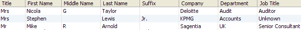
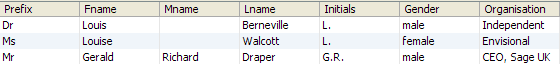
Merge Data Streams Configuration
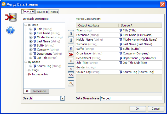
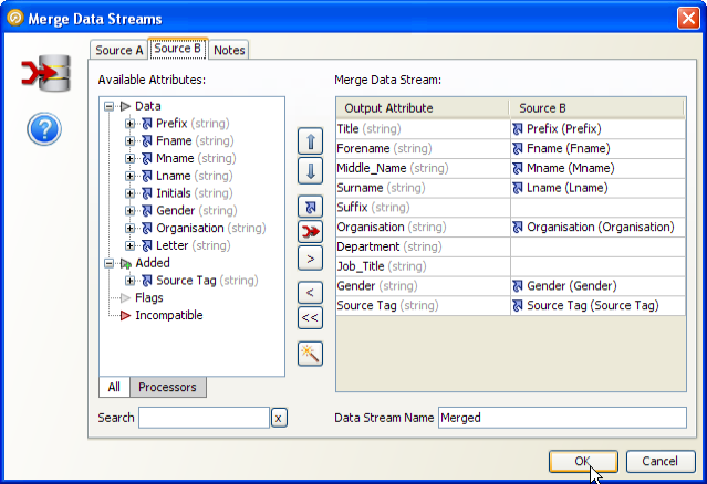
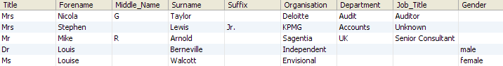
1.3.8.2 Reader
A Reader is a special type of processor that is used to read data at the beginning of a process. Readers may connect to any of the following sources of data:
-
Staged data (that is, a snapshot of data - either present in the repository or not - or output data that has been written by another process);
-
A Data Interface (which can then be redirected to different sources of data using Mappings);
-
A set of Reference Data;
-
A Real time provider of messages (for example, the inbound interface of a Web Service)
A process must contain at least one Reader, but may contain many Readers, if matching data from multiple sources.
Readers are used at the beginning of processes in order to select the sources of data that you are intending to work with in the process, and any selection and reordering of data attributes from that data source that are specific to the process you are intending to create. For example, for the purposes of a specific process, you may want to select only the name and address fields from a data source, and you may want to reorder them for the purpose of display throughout your process.
A Reader is automatically added to a process for you, since a process must always have at least one Reader.
Select the Type of data that you want to read from the following options:
-
Staged data - that is, a snapshot of data, or the named output of another process, in the EDQ repository
Note:
The snapshot does not necessarily have to exist in the repository. You may be intending to run the process in streaming mode, meaning the source data will not be copied into the repository. -
Data Interface - that is, a configured source-independent interface of a set of data attributes
-
Reference Data - that is, a set of reference data that exists in the EDQ repository
-
Real time provider - that is, a direct connection to a real time source of messages
Select the Source of data from the available sources of the selected type.
All the available attributes in the data appear in the left pane. Select those that you want to work with in the process by using the arrow buttons to select, and de-select attributes:
| Arrow Button | Description |
|---|---|
| Selects the attributes highlighted in the left-hand pane as inputs to the process. | |
| Selects all available attributes as inputs. | |
| De-selects the selected inputs in the right-hand pane. | |
| De-selects all inputs. |
In the right-hand pane, the attributes that you have chosen to work with may be re-ordered by drag-and-drop.
The order that you specify in the Reader will be used to display results throughout the process.
Note:
If you know you are not intending to work with all the attributes of a given set of data, it is a good idea to exclude them in the Reader. This will make configuring your processors and browsing your results much more straight-forward as only the attributes you are interested in will be displayed.None
The Reader is a necessary part of any process, whatever the remit of that process is. Some processors are not suitable for certain types of execution, however. For example, it is not possible to match and consolidate data from numerous sources in a real time response process, but selecting a Real time Reader Source (as above) places no restrictions on the processors that are available for configuration, as the execution of a process is driven from how its Reader(s) and Writer(s) are configured.
In general, EDQ is designed for three modes of execution:
-
Batch execution, where a set of records in one or more data sources is processed in batch.
-
Real time monitoring execution, where EDQ acts as a data quality probe for a data source, monitoring incoming records for quality as they are created, but where no real time response to each record is expected.
-
Real time response execution, where EDQ processes records, and passes them back along with extra data, on a real time response interface.
Each processor in the library is listed with the execution modes that can be sensibly used with that processor.
The results browser for a Reader displays all the records present in the underlying data store once a process has been run.
The Reader does not provide any output filters. All records are read from the specified source and made available to the remainder of the process.
The following example shows the records that are read from the example Service Management data in the example Service Management Project.
In this case, the Reader was configured to read all the data attributes from the source, without changing their order. No further processing has yet been defined:
| CU_NO | CU_ACCOUNT | TITLE | NAME | GENDER | BUSINESS |
|---|---|---|---|---|---|
| 13810 | 00-23603-JD | Ms | Lynda BAINBRIDGE | F | Filling Station |
| 13815 | 00-23615-PB | William BENDALL | M | Edge Kamke & Ellis Ltd | |
| 13833 | 00-23624-PB | Ms | Karen SMITH | F | |
| 13840 | 00-23631-JD | Miss | Patricia VINER | Catchpole Engineering Products | |
| 13841 | 00-23642-SH | Mr | Colin WILLIAMS | M | Sanford Electical Co |
1.3.8.3 Writer
A Writer is a special type of processor used to write out records to a Staged Data table, Data Interface, Reference Data, or Real time consumer (for real time responses). You can select the attributes you choose to write, and map them to attributes with a different name in your Staged Data table, Data Interface, or real time response.
Once data is in a Staged Data table, it may exported to a Data Store, used in another process, or used in a lookup.
Use a Writer or Writers at the end of a process to report on its results, or to return a response to an external system.
For example:
-
From a batch auditing process, you might write out all valid records to one table, and all invalid records to another table.
-
From a batch cleansing process, you might write out the records that you are intending to migrate to a new system into a Staged Data table, and then check, or recheck, that data in other processes before export.
-
From a real time cleansing process, you might use a Writer to issues responses to each incoming record, with various corrections made.
Any attributes that you want to write to a Staged Data table, to Reference Data, to a Data Interface, or as a real time response.
Note:
If you are writing to Reference Data, the data that you are writing must conform to any uniqueness constraints defined in the Reference Data set. For example, if generating a Reference Data set with a uniqueness constraint on a lookup column, make sure that the data you write does not have duplicate values in that column. You may need to use the Group and Merge processor before writing the data to ensure that the data will write correctly. For information about configuring Reference Data, see Adding Reference Data. MoreNote that unlike most other processors, the Writer does not launch its configuration dialog when it is connected on the Canvas. This is because Writers are often connected to multiple streams. To launch the Writer configuration dialog, double-click on the processor on the Canvas.
Select the Type of target that you want to write to:
-
Staged data, where you want to write to a table in the EDQ repository, or directly to an external Data Store.
-
Data interface, where you want to choose the target of the data in job configuration rather than in the process, using data interface mappings.
-
Reference data, where you want to use the data in the process to write Reference Data that you will then edit in Director and use in other processors.
-
Real time consumer, where you have a configured Real time consumer that will pick up the response messages.
Then, choose which attributes to write, from the selection on the left. Selected attributes for writing appear in the middle pane for mapping to the target. There are two options above the attribute list to show more information - Show Actual Attributes, which will display the actual attribute name where you are using the latest version of an attribute, and Show Data Types, which will display the data types of the attributes.
The Staged Data table or Reference Data you can write to can either be:
-
Created using the New button (this creates a Staged Data table or Reference Data that corresponds to the selected set of attributes; the attributes may be renamed if required)
-
Selected from the drop down of existing Staged Data tables or Reference Data.
Use the Auto button at the bottom of the screen to map all selected attributes directly to a selected Staged Data table or Reference Data.
Use the Clear button to clear all mappings between selected attributes and attributes in the Staged Data table or Reference Data. (Note that the attributes and columns remain until deleted.)
Click and drag attributes in the middle column to reorder them.
It is also possible to edit the definition of the Staged Data table or Reference Data from the Project Browser or by launching the data editor from the Writer Configuration dialog using the Edit button, ![]() .
.
| Execution Mode | Supported |
|---|---|
| Batch | Yes |
| Real time Monitoring | Yes |
| Real time Response | Yes |
The data written by the Writer can be viewed in the Results Browser.
In this example, a number of invalid records are written to a Staged Data table called Quarantine output:
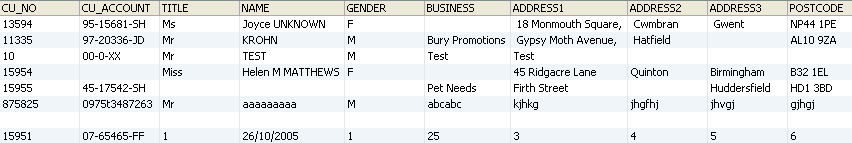
Description of the illustration ''examplewriter.png''
1.3.9 Text Analysis Processors
Text analysis processors offer advanced tools for understanding and improving data stored in text fields. Typically, this data might need to be analyzed and its contents understood, in order to transform it into a new structure. For example, it may be necessary to transform address data that has been manually entered in loosely structured address fields into a more suitable structure for matching. Or, if you are migrating data from several systems to a new system, it may be that the required structure of the data in the new system is different from your sources.
There are two text analysis processors: the Phrase Profiler, and Parse.
The Phrase Profiler analyzes text fields for their contents, and returns the most common words and phrases in the data.
Parse allows you to construct and use rules to understand the contents in full, to validate the data, and to transform it to a new structure if required.
1.3.9.1 Character Tag
The Character tag is used in the first step of tokenization to assign each character in the data (identified by Unicode character reference) a given tag - for example all lower case letters might be assigned a character tag of 'a'.
1.3.9.2 Character Type
The Character type is used to split up data. In general, a change of character type causes a split into separate base tokens. For example, the string 'deluxe25ml' will be split into three base tokens - 'deluxe', '25' and 'ml'. These three base tokens will then be tagged according to their character and group tags.
The exception to this rule is that, by default, a change of character type from ALPHA_UPPERCASE to ALPHA_LOWERCASE does not cause a split in tokens. This is in order to preserve tokens that are in proper case - for example, not to split 'Michael' into two tokens ('M' and 'ichael').
The user can change this behavior by selecting the option to Split Upper to Lower case.
The user can also choose to keep all strings of alpha characters together by de-selecting the option to Split Lower to Upper case. This would have the effect of keeping 'DelUXE' as one token.
Also, certain characters may be marked with a type of either WHITESPACE or DELIMITER. These characters can be ignored in later rules for matching sequences of tokens. For example, in Reclassify or Resolve, if you want to match a pattern of <Token A> followed by <Token B>, you may not care whether or not there are whitespace or delimiter characters in between them.
The possible character types are NUMERIC, CONTROL, PUNCTUATION, SYMBOL, ALPHA_UPPERCASE, ALPHA_LOWERCASE and UNDEFINED.
1.3.9.3 Classify
The Classify sub-processor of Parse adds semantic meaning to the data by classifying tokens using rules.
Classify applies a number of Token Checks to the data, where each Token Check attempts to classify either Base Tokens, or sequences of Base Tokens, with a given meaning (for example, as a 'Postcode').
Within each Token Check, a number of rules may be used. Each rule uses a method of checking the data - for example matching the data against a list - and classifies the data that passes the check with a tag, corresponding to the name of the Token Check, and a confidence level (Valid or Possible).
Note that a given token will have many possible semantic meanings if it matches more than one Token Check. For example, the token 'Scott' may be classified as both a 'valid Forename' and as a 'valid Surname'. The Select sub-processor will later attempt to assign each token its best meaning from all the possibilities available, based on the context of the token within the data.
Classification is a vital part of parsing. Use classification rules to give meaning to the tokens (such as numbers, words and phrases) that appear in your data. The patterns of token classifications may be used in later steps to validate the data, and to resolve it into a new output structure if desired.
Classification rules will often use lists of words and phrases that are created from the data itself using the results of the Phrase Profiler and Frequency Profiler.
The Configuration window for Classify has two tabs - Token Checks, and Attributes.
Use the Token Checks tab to configure your classification rules, in the form of a number of checks for different tokens.
Use the Attributes tab to associate these Token Checks with the input attributes.
A Token Check comprises one or more rules for identifying data that has a given semantic meaning.
Commonly, a Token Check will consist of a single rule that identifies data using a list of values. For example, for a 'Title' Token Check, a single List Check rule might be used with a reference list of valid titles (such as 'Mr', 'Mrs', 'Ms' etc.)
However, more complex types of Token Check may be configured. This is often necessary where it is not possible to maintain lists of valid token values (for example, because there are too many possible values).
For example, the following Token Checks might be used when parsing people's names:
Table 1-118 Token Check: Forename
| Order | Rule Type | Condition | Decision |
|---|---|---|---|
|
1 |
List Check |
Matches list of common Forenames |
Valid |
|
2 |
Base Token Check |
Matches base token tag: A |
Possible |
Table 1-119 Token Check: Surname
| Order | Rule Type | Condition | Decision |
|---|---|---|---|
|
1 |
List Check |
Matches list of common Surnames |
Valid |
|
2 |
List Check |
Matches list of bad data tokens |
Invalid |
|
3 |
Attribute word length check |
Is more than 2 words in length |
Invalid |
|
4 |
Base Token Check |
Matches base token patterns: A (for example, 'Davies') A-A (for example, 'Smith-Davies') A_A (for example, 'Taylor Smith') |
Possible |
Note:
By default, all token checks are displayed. To filter them by the attribute to which they are applied, select the required attribute in the drop-down selection field above the list of tokens.Importantly, the rules within each Token Check are processed in order, meaning that if a higher rule in the Check is hit, lower rules will not be. So, for example, if the token 'Smith' has been classified as a Valid Surname using the top rule in the Surname Token Check above, it will not be classified as a Possible Surname by rule 4. Equally, if the token 'Unknown' has been blocked from classification as a Surname by rule 2, it will not be classified as a Possible Surname by rule 4.
In this way, it is possible to use Token Checks either positively or negatively. You can positively identify Valid or Possible tokens by matching lists, or you can negatively identify tokens that are Invalid, and only classify the remaining tokens as Valid or Possible.
The following types of classification rule are available within each Token Check:
Table 1-120 Classification Rules within Token Check
| Rule Type | Description |
|---|---|
|
List Check |
Checks across the attribute for any data that matches a List or Map. Where a Map is used, it is possible to perform replacements (standardizations) of matched tokens within the parser. If the Use replacements in output option is checked, the mapped value (where present) will be used in preference to the matched value in output. It is possible to specify a Reference Data set of Noise Characters; that is, characters to remove before attempting to match the list. |
|
Regular Expression Check |
Checks across the attribute for any data that matches a Regular Expression. |
|
Attribute Completeness Check |
Checks that the attribute contains some meaningful data (other than whitespace). |
|
Pattern Check |
Checks across the attribute for any Base Tokens that match a Character Pattern, or list of Character Patterns. This check is case sensitive. |
|
Attribute Character Length Check |
Checks the length of the data in the attribute according to a number of characters. |
|
Attribute Word Length Check |
Checks the length of the data in the attribute according to a number of words. |
|
Base Token Check |
Checks across the attribute for tokens that match a given Base Token Tag (such as 'A', or patterns of tokens that match a given pattern of Base Token Tags (such as 'A-A'). See the note on Special Characters below. |
Note that if you want to check for Base Token patterns including full stops, such as 'A.A.A' for values such as 'www.example.com', the full stops must be entered with a \ before them in the Reference Data, as the full stop is a special character in parsing. So, for example, to check for a Base Token pattern of 'A.A.A', you must enter 'A\.A\.A'.
Note: In order to tag a full stop as its own character (.), rather than with the default base token tag of P, you would need to edit the default Base Tokenization Map used in parsing.
Applying Token Checks to Attributes
To apply Token Checks to Attributes, use the Attributes tab, and use the arrow buttons (or drag-and-drop) to select and de-select Token Checks from Attributes. You will commonly want to apply the same Token Check to many Attributes, and many Token Checks per Attribute.
The results of Phrase Profiling are often useful in order to determine which Token Checks to apply to which Attributes, as it is easy to see which types of tokens appear where.
Note that if you have added any Token Checks that are not associated with any Attributes (and which therefore will have no effect), you are warned before exiting the Classify configuration dialog.
In this example, TITLE and NAME attributes are parsed, using a number of Token Checks. The TITLE attribute is simply checked for Title tokens. The NAME attribute is checked for Forenames, Surnames, Initials, Name Qualifiers, and Name Suffixes.
The Token Checks View shows the summary of each Token Check within each attribute, with the counts of the distinct classified token values at each classification level (Valid and Possible):
| Attribute | Token Check | Valid | Possible |
|---|---|---|---|
|
NAME |
<Forename> |
772 |
72 |
|
NAME |
<Initial> |
19 |
0 |
|
NAME |
<Surname> |
1623 |
70 |
|
NAME |
<Qualifier> |
7 |
0 |
|
NAME |
<Suffix> |
0 |
0 |
|
TITLE |
<Title> |
10 |
0 |
It is then possible to drill down to see the distinct tokens, and the number of records that contain each token. For example, you could drill down on the tokens that were classified as valid forenames.
Drilling down again takes you to the records that contain the relevant token. Note that it is possible that a single record may contain the same token twice (but will only be counted once).
The Classification View displays all of the token patterns (descriptions of the data) generated after the classification step. Note that for a given input record, multiple token patterns may be generated, because the same token may be classified by different checks. This means that the same record may appear under several of the token patterns.
Note that some of the records that have the most common token pattern (for example, <valid Title><valid Forename>_<valid Surname>) will also have the second most common token pattern (for example, <valid Title><valid Surname>_<valid Surname>). As the former pattern is more common, however, it can be selected as the most likely description of these records using pattern frequency selection in the Select sub-processor. Alternatively, we can use context-sensitive Reclassification rules (see Reclassify) to add the intelligence that a token in between a Title and Surname is unlikely to be another surname, even if it passes the context-free token check.
The Unclassified Tokens View shows a view of the number of (base) tokens in each attribute that have not been classified by any of the token checks. This is useful to find values that may need to be added to lists used for classification.
From the example above, we might have the following view of unclassified tokens:
Drilling down shows each distinct token, and its frequency of occurrence. For example, we can drill down on the 55 unclassified tokens in the NAME field above. This may reveal some unusual characters, some dummy values, and some mis-spellings.
Table 1-123 Drilling down on Unclassified Tokens
| Token | Frequency | No. records |
|---|---|---|
|
# |
13 |
13 |
|
- |
12 |
12 |
|
TEST |
4 |
4 |
|
Test |
3 |
3 |
|
Cluadia |
1 |
1 |
|
DO |
1 |
1 |
|
WHUR |
1 |
1 |
We can now use this view to add to the classification lists, or create new lists (for example, to create a list to recognize dummy values).
The next (optional) step in configuring a Parse processor is to Reclassify data.
1.3.9.4 Group Tag
The Group tag is used in the second step of tokenization to group sequences of character tags with the same Group tag.
Sequences of character tags with the same group tag, and the same character type, will be grouped to form a single token.
For example, the first phase of tokenization might tag the data "103" as "NNN", using character tags, but as there are three characters with the same group tag ('N') and the same character type (NUMERIC), in sequence, these are grouped to form a single Base Token ("103"), with a Base Token Tag of 'N'.
Note that the behavior for ALPHA characters is slightly different, as the user can choose whether or not to split tokens where there is a sequence of lower case and upper case letters. By default, tokens are split on transition from lower case to upper case, but not from upper case to lower case. For example, the data "Michael" has the sequence of character tags 'Aaaaaaa', but has a transition in character type from ALPHA_UPPERCASE to ALPHA_LOWERCASE after the first letter. If the user keeps the default setting of the Split Upper to Lower Case option as not set, this will be grouped to form a single Base Token ("Michael") with a Base Token tag of 'A', as the character tags 'a' and 'A' both share the same group tag, and because the user is not splitting data on the transition of character type.
1.3.9.5 Input
The Input sub-processor of Parse is used to select the input attributes to the parsing process.
The sub-processor also allows you to configure Dashboard publication options, and add any notes on the processor (for example, authorship details if designing a parser for distribution to other users).
Select the input attribute(s) for the Parse processor using the standard input screen.
1.3.9.6 Map
The Map sub-processor of Parse is used to map the selected input attributes to the internal attributes used by the Parse processor.
Using internal attributes allows a Parse processor to be developed and configured independently of the actual names of the input attributes. This is useful because the same Parse processor can be re-used with multiple different data sources, which may provide differently named input attributes, simply by mapping the new input attributes to the existing internal attributes. There is no need to reconfigure any other options (such as which classification and reclassification rules to apply to which attributes).
Each internal attribute has a name (such as Title, Forename, Surname and so on) and a tag (usually a1, a2, a3 and so on). Tags can be used in the resolution phase of parsing, to allow the Parse processor to distinguish between token patterns which originate from different input patterns. See Using Attribute Tags for more details.
The attributes required by the parser are displayed on the left. Map your selected input attributes to these attributes in the right-hand column.
1.3.9.7 Parse
The Parse processor is an extremely powerful tool for the understanding and structural improvement of data. It allows you to analyze and understand the semantic meaning of data in one or many attributes, by applying both manually configured business rules, and artificial intelligence. It then allows you to use that semantic meaning in rules to validate and optionally restructure the data. For example, Parse allows you to recognize names data that is wrongly captured in address attributes, and optionally map it to new attributes in a different structure.
The Parse processor can be configured to understand and transform any type of data. For an introduction to parsing in EDQ, see the Parsing Concept Guide. More
The Parse processor has a variety of uses. For example, you can use Parse to:
-
Apply an improved structure to the data for a specific business purpose, such as to transform data into a structure more suitable for accurate matching.
-
Apply structure to data in unstructured, or semi-structured format, such as to capture into several output attributes distinct items of data that are all contained in a single Notes attribute.
-
Check that data is semantically fit for purpose across a number of attributes, either on a batch or real-time basis.
-
Change the structure of data from a number of input attributes, such as to migrate data from a number of different source formats to a single target format.
The Parser runs in several steps. Each step is fully explained in the Configuration section below. However, the processing of the parser can be summarized as follows:
Input data >
-
Tokenization: Syntactic analysis of data. Split data into smallest units (base tokens)
-
Classification: Semantic analysis of data. Assign meanings to tokens
-
Reclassification: Examine token sequences for new classified tokens
-
Pattern Selection: Select the best description of the data, where possible
-
Resolution: Resolve date to its desired structure and give a result
> Output data and flags
To understand how the Parse processor works as a whole, it is useful to follow an example record through it. In this example, we are parsing an individual name from three attributes - Title, Forenames, and Surname.
Example Input Record
The following record is input:
| Title | Forenames | Surname |
|---|---|---|
| Mr | Bill Archibald | SCOTT |
Tokenization
Tokenization tokenizes the record as follows, recognizing the tokens 'Mr', 'Bill', 'Archibald' and 'SCOTT' and assigning them a token tag of <A>. It also recognizes the space between 'Bill' and 'Archibald' as a token and assigns it a token tag of <_>. Note that Tokenization always outputs a single pattern of base tokens. In this case, the pattern is as shown below (from the Tokenization view):
| Title | Forenames | Surname |
|---|---|---|
| <A> | <A>_<A> | <A> |
Classification
Classification then classifies the tokens in the record using classification rules with lists of names and titles. As some of the names appear on multiple lists, some of the tokens are classified in multiple ways - for example, the token 'Archibald' is classified both as a <possible forename> and as a <possible surname>, and the token 'SCOTT' is classified both as a <possible forename> and as a <valid surname>. As a result, Classification outputs multiple classification patterns, as shown below in the Classification view:
| Title | Forenames | Surname |
|---|---|---|
| <valid title> | <valid forename>_<possible_surname> | <possible forename> |
| <valid title> | <valid forename>_<possible_forename> | <possible forename> |
| <valid title> | <valid forename>_<possible_surname> | <valid surname> |
| <valid title> | <valid forename>_<possible_forename> | <valid surname> |
Reclassification
As above, we now have multiple descriptions of the data. However, we might decide to apply the following Reclassification rule to the Forenames attribute to denote that because the token 'Archibald' follows a valid forename, we can be confident that it represents a middle name:
| Name | Look for | Reclassify as | Result |
|---|---|---|---|
| Middle name after Forename | <valid forename>(<possible forename>) | middlename | Valid |
This rule acts on the pattern '<valid forename>(<possible forename>)' in the Forenames attribute, which affects the second and fourth classification patterns above. As Reclassification adds new patterns but does not take away existing ones, we now have the original four patterns and two new ones, as shown in the following table:
| Title | Forenames | Surname |
|---|---|---|
| <valid title> | <valid forename>_<possible_surname> | <possible forename> |
| <valid title> | <valid forename>_<possible_forename> | <possible forename> |
| <valid title> | <valid forename>_<possible_surname> | <valid surname> |
| <valid title> | <valid forename>_<valid_middlename> | <valid surname> |
| <valid title> | <valid forename>_<valid_middlename> | <possible forename> |
| <valid title> | <valid forename>_<possible_forename> | <valid surname> |
Note:
The Reclassification view will only show the patterns that have been pre-selected for entry into the Selection process. Pre-selection is a non-configurable first step in the selection process which eliminates patterns containing too many unclassified tokens. The pre-selection process first surveys all the patterns generated so far, and determines the minimum number of unclassified tokens present in any one pattern. Next, any patterns with more than that number of unclassified tokens are eliminated. In the example above, none of the patterns contain any unclassified tokens, so the minimum number of unclassified tokens is zero. Since none of the patterns contain more than zero unclassified tokens, none of the patterns are eliminated in the pre-selection process.Selection
Selection now attempts to pick the best overall pattern from the six possibilities. In this case, we can see that the fourth pattern above is the strongest as all of its token classifications have a result of 'valid'. By scoring each of the patterns using the default selection rules, therefore, the first pattern is selected and displayed in the Selection view:
| Title | Forenames | Surname |
|---|---|---|
| <valid title> | <valid forename>_<valid_middlename> | <valid surname> |
Resolution
If we accept that the selected pattern is a good description of the record, we can then resolve the pattern to output attributes, and assign a result. In this case, we can do this by right-clicking on the selected pattern above and selecting Resolve... to add an Exact resolution rule.
We use the default output assignments (according to the classifications made), and assign the pattern a Pass result, with a Comment of 'Known name format'.
After re-running Parse with this rule, we can see that the rule has resolved the input record:
| Id | Rule | Result | Comment | Count |
|---|---|---|---|---|
| 1 | Exact Rule | Pass | Known name format | 1 |
Finally, we can drill down to the record and see that data has correctly been assigned to output attributes according to the resolution rule:
| Title | Forenames | Surname | UnclassifiedData.Parse | title.Parse | forename.Parse | surname.Parse |
|---|---|---|---|---|---|---|
| Mr | Bill Archibald | SCOTT | Mr | Bill | SCOTT |
Parse is an advanced processor with several sub-processors, where each sub-processor performs a different step of parsing, and requires separate configuration. The following sub-processors make up Parse, each performing a distinct function as described below.
| Sub-processor | Description |
|---|---|
| Input | Allows you to select the input attributes to parse, and configure Dashboard publication options. Note that only String attributes are valid inputs. |
| Map | Maps the input attributes to the attributes required by the parser. |
| Tokenize | Tokenize analyzes data syntactically, and splits it into its smallest units (base tokens) using rules. Each base token is given a tag, for example <A> is used for an unbroken sequence of alphabetic characters. |
| Classify | Classify analyzes data semantically, assigning meaning to base tokens, or sequences of base tokens. Each classification has a tag, such as 'Building', and a classification level (Valid or Possible) that is used when selecting the best description of ambiguous data. |
| Reclassify | Reclassify is an optional step that allows sequences of classified and unclassified (base) tokens to be reclassified as a single new token. |
| Select | Select attempts to select the 'best' description of the data using a tuneable algorithm, where a record has many possible descriptions (or token patterns). |
| Resolve | Resolve uses rules to associate the selected description of the data (token pattern) with a Result (Pass, Review or Fail), and an optional Comment. It also allows you to configure rules for outputting the data in a new structure, according to the selected token pattern. |
The Parser offers two modes of execution in order to provide optimized performance where some of the results views are not required.
The two modes are:
-
Parse and Profile
-
Parse
Parse and Profile (the default mode) should be used when first parsing data, as the parser will output the Token Checks and Unclassified Tokens results views, which are useful when still in the process of defining the parsing rules, by creating and adding to lists used for classification.
Parse mode should be used when the classification configuration of the parser is complete, and optimal performance is needed. Note that the Token Checks and Unclassified Tokens views are not produced when running in this mode.
All options are configurable within each sub-processor.
Data Attributes
The output data attributes are configurable in the Resolve sub-processor.
Flags
| Flag attribute | Purpose | Possible Values |
|---|---|---|
| [Attribute name].SelectedPattern | Indicates the selected token pattern for the record | The selected token pattern |
| [Attribute name].BasePattern | Indicates the base token pattern for the record, output from tokenization (if using the parser purely to generate this pattern) | The base token pattern |
| ParseResult | Indicates the result of the parser on the record. | Unknown/Pass/Review/Fail |
| ParseComment | Adds the user-specified comment of the record's resolution rule. | The comment on the resolution rule that resolved the record |
The Parse processor's results may be published to the Dashboard.
The following interpretation of results is used by default:
| Result | Dashboard Interpretation |
|---|---|
| Pass | Pass |
| Review | Warning |
| Fail | Alert |
| Execution Mode | Supported |
|---|---|
| Batch | Yes |
| Real time Monitoring | Yes |
| Real time Response | Yes |
The Parse processor produces a number of views of results as follows. Any of the views may be seen by clicking on the Parse processor in the process. The views may also be seen by expanding the Parse processor to view its sub-processors, and selecting the sub-processor that produces the view.
Base Tokenization View (produced by Tokenize)
This view shows the results of the Tokenize sub-processor, showing all the distinct patterns of Base Tokens across all the input attributes. The patterns are organized by frequency.
Note:
Each record has one, and only one, base token pattern. Many records have the same base token pattern.| Statistic | Meaning |
|---|---|
| For each input attribute | The pattern of base tokens within the input attribute
Note that rows in the view exist for each distinct base token pattern across all attributes |
| Count | The number of records with the distinct base token pattern across all the input attributes |
| % | The percentage of records with the distinct base token pattern across all the input attributes |
Token Checks View (produced by Classify)
This views shows the results of the Classify sub-processor, showing the results of each token check within each input attribute.
| Statistic | Meaning |
|---|---|
| Attribute | The attribute to which the token check was applied |
| Classifier | The name of the token check used to classify tokens |
| Valid | The number of distinct tokens that were classified as Valid by the token check |
| Possible | The number of distinct tokens that were classified as Possible by the token check |
Drill down on the Valid or Possible statistics to see a summary of the distinct classified tokens and the number of records containing them. Drill down again to see the records containing those tokens.
Unclassified Tokens View (produced by Classify)
| Statistic | Meaning |
|---|---|
| Attribute | The input attribute |
| Unclassified Tokens | The total number of unclassified tokens in that attribute |
Drill down on the Unclassified Tokens to see a list of all the unclassified tokens and their frequency. Drill down again to see the records containing those tokens.
Classification View (produced by Classify)
This view shows a list of all the generated token patterns after classification (but before reclassification). There may be many possible patterns for each input record.
| Statistic | Meaning |
|---|---|
| For each input attribute | The pattern of tokens across the attribute.
Note that rows in the view exist for each distinct token pattern across all attributes. |
| Count | The number of records where the token pattern is a possible description of the data. Note that the same record may have many possible token patterns in this view, and each token pattern may describe many records. |
| % | The Count expressed as a percentage of all the possible token patterns across the data set. |
Reclassification Rules View (produced by Reclassify)
This view shows a list of all reclassification rules, and how they have affected your data.
| Statistic | Meaning |
|---|---|
| Rule Id | The id of the reclassification rule. The ids are auto-assigned. The id is useful where you have dependencies between rules - see the Precedents statistic below. |
| Rule Name | The name of the reclassification rule. |
| Attribute | The attribute to which the reclassification rule was applied. |
| Look for | The token pattern used to match the rule |
| Reclassify as | The target token of the reclassification rule |
| Result | The classification level (valid or possible) of the reclassification rule |
| Records affected | The number of records affected by the rule |
| Patterns affected | The number of classification patterns affected by the rule |
| Precedents | The number of other reclassification rules that preceded this rule before it could operate. For example, if you reclassify the <A> as <B> in one rule, and <B> to <C> in another rule, the first rule is a precedent of the second. Note that even reclassification rules that did not affect any records may have precedents, as these are calculated logically. |
Reclassification View (produced by Reclassify)
This view shows a list of all the generated token patterns after reclassification (but before selection). There may be many possible patterns for each input record. The view presents all of the possible patterns and their frequency across the whole data set, before the Select step attempts to select the best pattern of each input record.
Note:
The data in this view may itself be used to drive which pattern to select; that is, it is possible to configure the Select step to select the pattern for a record by assessing how common it is across the data set. See the configuration of the Select sub-processor.| Statistic | Meaning |
|---|---|
| For each input attribute | The pattern of tokens across the attribute.
Note that rows in the view exist for each distinct token pattern across all attributes. |
| Count | The number of records where the token pattern is a possible description of the data. Note that the same record may have many possible token patterns in this view, and each token pattern may describe many records. |
| % | The Count expressed as a percentage of all the possible token patterns across the data set. |
Selection View (produced by Select)
After the Select step, each input record will have a selected token pattern.
This view shows a view of the selected patterns across the data set, and their frequency of occurrence.
Note:
Where the selection of a single token pattern to describe a record is not possible, because of ambiguities in selection, the pattern with the ambiguity (or ambiguities) is shown along with the number of records that had the same ambiguity; that is, the same set of potential patterns that selection could not choose between| Statistic | Meaning |
|---|---|
| For each input attribute | The pattern of tokens across the attribute
Note that rows in the view exist for each distinct token pattern across all attributes. |
| Exact rule | The numeric identifier of the exact resolution rule (if any) that resolved the token pattern |
| Fuzzy rule | The numeric identifier of the fuzzy resolution rule (if any) that resolved the token pattern |
| Count | The number of records where the token pattern was selected as the best description of the data |
| % | The percentage of records where the token pattern was selected |
Resolution Rule View (produced by Resolve)
This view shows a summary of the resolutions made by each Resolution Rule. This is useful to check that your rules are working as desired.
| Statistic | Meaning |
|---|---|
| ID | The numeric identifier of the rule as set during configuration. |
| Rule | The type of rule (Exact rule or Fuzzy rule) |
| Result | The Result of the rule (Pass, Review or Fail) |
| Comment | The Comment of the rule |
| Count | The number of records that were resolved using this rule. Click on the Additional Information button in the Results Browser to show this as a percentage. |
Result View (produced by Resolve)
| Statistic | Meaning |
|---|---|
| Pass | The total number of records with a Pass result |
| Review | The total number of records with a Review result |
| Fail | The total number of records with a Fail result |
| Unknown | The number of records where Parse could not assign a result |
The following output filters are available from the Parse processor:
-
Pass - records that were assigned a Pass result
-
Review - records that were assigned a Review result
-
Fail - records that were assigned a Fail result
-
Unknown - records that did not match any resolution rules, and therefore had no distinct result
In this example, a complete Parse configuration is used in order to understand the data in a single NAME attribute, and output a structured name:
Base Tokenization view
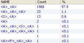
Description of the illustration ''exampleparsetokenizationsumm.png''
Token Checks view
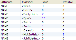
Description of the illustration ''exampleparseclassifysumm.png''
Classification view
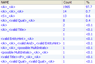
Description of the illustration ''exampleparseclassificationsumm.png''
Unclassified Tokens view
Description of the illustration ''exampleparseunclassifiedtokens.png''
Reclassification Rules view
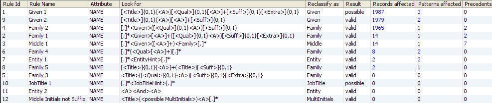
Description of the illustration ''exampleparsereclassificationrules.png''
Reclassification view
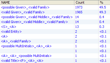
Description of the illustration ''exampleparsepreselection.png''
Selection view
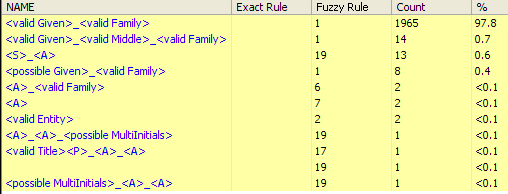
Description of the illustration ''exampleparsepostselection.png''
Resolution Rule view
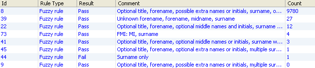
Description of the illustration ''exampleparseresolutionview.png''
Results view
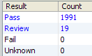
Description of the illustration ''exampleparseresultsview.png''
Drill down on Pass results
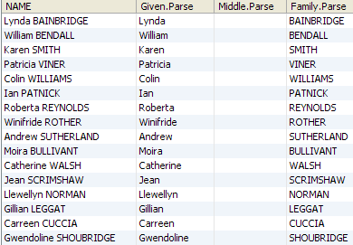
Description of the illustration ''exampleparsedd.png''
1.3.9.8 Phrase Profiler
The Phrase Profiler analyzes a number of attributes and searches for common words and phrases.
The returned words and phrases are returned in order of their frequency within all the input attributes.
The Phrase Profiler is a quick way of discovering the most frequent and significant words and phrases in the data, and where they occur. You can then use the results of phrase profiling to drive the configuration of the Parse processor. For example, you can add the words and phrases that were found to Reference Data lists used to classify data, and, by seeing which words and phrases occur in which attributes, work out which token checks to apply to which attributes.
The Phrase Profiler is therefore an important tool to use when understanding the content of text fields, especially when you may need to improve or otherwise change the structure of the data (for example, for a data migration).
The following table describes the configuration options:
| Configuration | Description |
|---|---|
| Inputs | Specify any string attributes that you want to analyze for common words or phrases. |
| Options | Specify the following options:
|
| Outputs | Describes any data attribute or flag attribute outputs. |
|
Data Attributes |
None. |
|
Flags |
None. |
| Execution Mode | Supported |
|---|---|
| Batch | Yes |
| Real time Monitoring | Yes |
| Real time Response | No |
A large dataset containing free text will typically contain a large number of distinct phrases with only a few of them being significant in understanding the content of the dataset.
The Phrase Profiler provides two main settings to help eliminate insignificant results: the Cutoff frequency and the Allowable variation.
Typically, the Phrase Profiler will generate a relatively small collection of phrases that occur in a large number of records and are potentially significant, together with a very large number of phrases that occur in a small number of records and so are less significant. You may want not to include the less frequent phrases in the results. As the absolute cutoff frequency varies depending on the size of the dataset, it is convenient to express the Cutoff frequency setting as a frequency per million input records.
Where a phrase consists of many words (or a substring consists of many characters), longer phrases will include shorter phrases, so that data that includes the phrase 'Newcastle Upon Tyne' will also include at least the same number of sub-phrases 'Newcastle Upon' and 'Upon Tyne'.
If the two sub-phrases occur with exactly the same frequency as the full phrase and there is no variation in their frequencies, then the full phrase is significant (a 'top-level phrase') and the sub-phrases are not. The sub-phrases are therefore excluded from the results.
If the sub-phrases occur more frequently than the full phrase, however, then they become more interesting and the variation in frequency between a phrase and a sub-phrase is a measure of the independent significance of the sub-phrase. So you may specify an Allowable variation to remove sub-phrases with a variation in frequency that is below this value. Again, as the absolute variation varies depending on the size of the dataset, it is convenient to express the Allowable variation setting as a variation per million input records.
Consider the following parameters:
-
1 million records are analyzed by the Phrase Profiler
-
The Cutoff frequency is set to 100 parts per million
-
The Allowable variation is set to 50 parts per million
-
There are 400 occurrences of the phrase 'Newcastle Upon Tyne'
-
There are 50 occurrence of the phrase 'Newcastel Upon Tyne'
The phrase 'Newcastle Upon Tyne' appears in the results but 'Newcastel Upon Tyne' does not because of the cutoff. The sub-phrase 'Upon Tyne' has a frequency of 450 and so is unaffected by the cutoff, but does not appear in the results because the frequency variation of 50 with its containing phrase is just within the allowable limit. If 'Upon Tyne' appeared in just one more record, anywhere within the data, then it would appear in the results as potentially significant. It is generally appropriate to set the Cutoff frequency and Allowable variation to the same value.
Sometimes it is useful to know if a phrase is a sub-phrase of something else or if it is a 'top level phrase'. In the above example, 'Newcastle Upon Tyne' may be a top-level phrase - in which case it presumably represents a city. However, if there were just one occurrence of the phrase 'Newcastle Upon Tyne Borough Council', and this occurrence is included in the results (not excluded by either the Cutoff or Allowable Variation options) then 'Newcastle Upon Tyne' would no longer be a top-level phrase and so may sometimes represent something other than a city. The Phrase Profiler flags top-level phrases in the results.
The following table describes the statistics produced by the profiler. The Phrase Profiler produces a summary view of its results, showing the words and phrases that were found in the input attributes in order of their frequency of occurrence.
| Statistic | Description |
|---|---|
| Size | .The size of the phrase, in number of words. |
| Top Phrase | .Indicates whether or not the phrase is a top-level phrase.See the note above explaining the Allowable variation setting. |
| Phrase | .The word or phrase that was found in the data. |
| Frequency | The number of occurrences of the phrase or word. Note that when drilling down to the data, you may see fewer records than this frequency, because the same phrase or word may occur more than once in some records. |
| [Attribute].freq | The number of occurrences of the phrase or word within each input attribute. |
In this example, Customer Name and Address data is analyzed with a view to parsing it to resolve any structural issues. The Phrase Profiler is run in order to find the most common words and phrases in the name and address attributes. The options are configured as follows:
-
Cutoff frequency: 5000
-
Allowable variation: 5000
-
Maximum words in a phrase: 10
-
Additional word delimiter: comma (,)
-
Word delimiter regular expression: not used
-
Ignore case?: No
For example, if the words 'Mr', 'Ms', 'Mrs' and 'Miss' are frequently occurring, and valid, Titles, so we might create a Reference Data list for classifying them in parsing. We can then sort the results by the Title attribute to find further values that occur.
1.3.9.9 Reclassify
The Reclassify sub-processor of Parse is an optional step that allows you to reduce the total number of different patterns of tokens in your data by recognizing sequences of classified and unclassified tokens, or tokens in a given context, and reclassifying them as a new token, with a given confidence level (valid or possible).
Use Reclassify wherever you have sequences of tokens that you want to consider together in output, and where you want to consider many similar patterns of tokens within an attribute as the same.
For example, when parsing addresses, you may see the following different patterns of data in an Address1 attribute after initial Classification:
<N>_<A>_<valid Road Hint> (for example, "10 Harwood Street")
<N>_<A>_<A>_<valid Road Hint> (for example, "15 Long End Road")
<A>_<valid Road Hint> (for example, "Nuttall Lane")
You may want to reclassify all these different sequences of tokens as valid Thoroughfares.
The Reclassify step is also useful because the Classify step does not consider context, other than which attribute a given piece of data is found in. You can use reclassification rules to reclassify tokens that were incorrectly classified within their context. For example, data such as "London Road" might be classified as <valid Town> <valid Road Hint>. You may choose to reclassify the sequence of tokens as a valid Thoroughfare, or to reclassify the <valid Town> part, by enclosing it in brackets in the rule, as a ThoroughfareName.
Each reclassification rule uses a structured expression to match patterns of tokens after Classification, and to reclassify a part of each matched pattern as a new token.
Rules may be easily enabled and disabled using the tick box in the Reclassify Rules dialog. Rules must be associated with the required input attributes in the Attributes tab.
The following table gives a guide to the syntax of the expressions used in reclassification:
| Characters | Use | Example |
|---|---|---|
| [ ] | Used to group a sequence of tokens in order to specify the number of times the sequence occurs. It is always followed by a range (enclosed in curly brackets) or by * or +.
If the group contains only a full stop [.] this means any token or tokens. |
[<A>]
Matches the token <A> |
| { } | Used to specify a range that expresses how many instances of the previous group (enclosed in square brackets) may occur in the pattern, in sequence. Ranges are specified with minimum and maximum numbers, separated by commas. | [<A>]{1,3}
Matches 1-3 occurrences of the token <A> in sequence [<A>]{2,2} Matches exactly 2 occurrences of the token <A> in sequence |
| ? | Used to denote that the group is optional. This has the same meaning as {0,1}; that is, this matches if the group does not appear, or appears only once. | [<title>]?
Matches if the title token does not appear, or appears once |
| + | Used instead of numbers in curly brackets (as above) to indicate that the previous group must occur at least once, but may occur any number of times. | [<A>]+
Matches any number of occurrences of the token <A> in sequence |
| * | Used instead of numbers in curly brackets to indicate that the previous group may occur any number of times, or not at all. | [.]* |
| [.] | Used to denote a wild card; that is, any token.
Use this together with rules on how many tokens you expect. For example, [.]* means any number of occurrences of any token. |
[.]*(<N><valid RoadHint>)[.]*
Reclassifies the sequence <N><valid RoadHint> wherever it occurs, without reclassifying any of the other tokens in the pattern |
| ( ) | Used to enclose the part of the pattern that you actually want to reclassify. Allows you to use pattern context in matching the Reclassification Rule, but not in the reclassification itself. | (<N><valid RoadHint>)<valid Town>
Reclassifies the sequence <N><valid RoadHint> provided it occurs before a valid Town token. |
| " " | Used to enclose exact data, where it is used in a rule instead of tokens. | - |
Note the following on reclassification rules:
-
Unless you use wild cards, each rule will attempt to match the whole of the token pattern in the attribute.
-
Rules do not need to be ordered, and will all be applied against the data set. Rules that are dependent on each other will be ordered automatically. For example, if you reclassify <A>_<valid Road Hint> as a <valid Thoroughfare>, and add an additional rule that reclassifies <N>_<valid Thoroughfare>, the latter rule will be processed after the first rule. Rules that are cyclical are not allowed. For example, it is not possible to reclassify <A> as <B> in one rule, and then <B> as <A> in another rule.
-
You may choose either to specify, or not specify, Base Tokens that represent either Delimiters or Whitespace, as driven from the configuration of the Tokenize step, in a reclassification rule. If you do not include them, the rule will ignore them when matching patterns against the rule. If you include them in the rule, they will have to match exactly. For example, the rule <N><valid Road Hint> will match both <N>_<valid Road Hint> and <N>___<valid Road Hint>, but the rule <N>_<valid Road Hint> would only match the former pattern.
-
You may choose either to specify, or not specify, the validity level of the tokens you are matching. For example, the rule <N><Road Hint> will match both <N><valid Road Hint> and <N><possible Road Hint>.
-
It is possible to use multiple reclassification rules that will reclassify different sequences of tokens to the same target token.
In this example, two reclassification rules are used to reduce the total number of patterns to resolve when parsing addresses by recognizing sequences of tokens that represent thoroughfares, such as "Acacia Avenue" and "London Road".
| Rule Name | Look For | Reclassify as | Result |
|---|---|---|---|
| Thoroughfare | [.]*([<A>]+<RoadHint>)[.]* | thoroughfare | valid |
| Reclassify towns in road names | [.]*([<Town>]+<RoadHint>)[.]* | thoroughfare | valid |
These two rules are both applied to an Address1 attribute. The results of the rules can be seen after running the process.
We can then drill down on the records and patterns affected to check that each rule is working correctly. Note that each reclassification rule may affect many patterns within the attribute it is applied to, and which in turn may affect many of the overall classification patterns (if parsing several attributes). As the same input record may have multiple classification patterns (as a single token may be classified in different ways), it may be that the same record may have multiple classification patterns affected by the same rule.
After the above reclassification rules have been applied, you can see the appearance of the <thoroughfare> token in a number of patterns in the Reclassification view.
The next step in configuring a Parse processor is to Select the best descriptions of your input data.
1.3.9.10 Resolve
Resolve is the final sub-processor of Parse. In this step, the selected token pattern of each record is used to drive the result of parsing (Pass, Review or Fail), and the way in which the data will be output, for example, in a new structure. All records with the same selected pattern will therefore be resolved in the same way.
The Resolve step is vital when using Parse either simply to validate data, or to transform data into a new structure.
For some types of data, it is often appropriate to configure the initial Parse processor with a simple set of rules, so that you can resolve the most frequent patterns and use simple mapping of tokens to output attributes to resolve the data into a new structure. You might then leave the remaining records in 'Review', and pass them on to a second Parse processor with a more complex configuration. This allows you to iterate round the processing of the second parser more quickly without affecting the records that you have already resolved.
There are three methods of resolving records in parsing:
-
Exact rules - which a single token pattern will match exactly. Records with that pattern will be resolved with a Result and an optional Comment, and will be output in the way dictated by the rule.
-
Fuzzy rules - which a number of token patterns may match. Records with a matching token pattern will be resolved with a single Result and optional Comment, and will be output in the way dictated by the rule.
-
Automatic extraction - where tokens from patterns that do not match any specific Exact or Fuzzy rules are automatically extracted to corresponding output attributes. No Result or Comment is associated with records with these unmatched patterns. Automatic extraction is used by default, but may be turned off if required.
The three different methods are processed in priority order; that is, Exact rules take precedence over Fuzzy rules, which take precedence over Automatic extraction. If a pattern matches an Exact rule, it will not be processed by any Fuzzy rules. If a pattern matches an Fuzzy rule, it will not be processed by Automatic extraction.
In some cases, if you have effectively resolved tokens to their desired output attributes by means of Classification and Reclassification, no specific resolution rules will be required; that is, Automatic extraction will be sufficient. However, it is often useful to be able to determine how to output data according to its specific token pattern. In this case, the type of specific resolution rules (Exact or Fuzzy) to use may depend on the volume of data you are processing, and the number of distinct token patterns that require resolution. If you have a small number of distinct patterns, you can resolve them simply using Exact rules. If you have a large number of distinct patterns, you may choose to resolve the most common patterns exactly, but use Fuzzy rules to resolve the remaining patterns.
Exact rules can only be created by browsing the selected token patterns in the Selection View (produced by the Select sub-processor), right-clicking on them, and selecting Resolve. Note that you can choose to resolve many patterns at once.
Use the arrow buttons at the top to move between token patterns.
Use the magic wand button to reset the mappings of tokens to their default attributes (that is, so that all tokens with a token tag that matches an output attribute name will be mapped to the matching output attribute, and all other tokens will be mapped to the UnclassifiedData output attribute, unless it has been deleted.)
You can add and remove output attributes by switching to the Output tab, adding and removing attributes, and switching back to the Exact tab to map the tokens from the patterns to these attributes.
When the parser is re-run, patterns that are resolved by an exact rule are displayed with a green background color, and with a reference to the rule identifier, in the Results Browser, to highlight the fact that they have been resolved.
Each Fuzzy rule uses a structured expression to match a number of token patterns. The structured expression is similar to that used in Reclassify, but with two differences:
-
You cannot use quote marks " " to match an Fuzzy resolution rule using the exact data in a given record, as resolution must occur per token pattern.
-
You cannot use normal parentheses ( ), as you can in reclassification rules to denote the part of the pattern that you want to reclassify. Resolution occurs against the whole pattern, across all input attributes.
The following table gives a guide to the syntax of the expressions used in Fuzzy resolution rules:
| Characters | Use | Example |
|---|---|---|
| [ ] | Used to group a sequence of tokens in order to specify the number of times the sequence occurs. It is always followed by a range (enclosed in curly brackets) or by * or +.
If the group contains only a full stop [.] this means any token or tokens. |
[<A>]
Matches the token <A> |
| { } | Used to specify a range that expresses how many instances of the previous group (enclosed in square brackets) may occur in the pattern, in sequence. Ranges are specified with minimum and maximum numbers, separated by commas. | [<A>]{1,3}
Matches 1-3 occurrences of the token <A> in sequence [<A>]{2,2} Matches exactly 2 occurrences of the token <A> in sequence |
| ? | Used to denote that the group is optional. This has the same meaning as {0,1}; that is, this matches if the group does not appear, or appears only once. | [<title>]?
Matches if the title token does not appear, or appears once |
| + | Used instead of numbers in curly brackets (as above) to indicate that the previous group must occur at least once, but may occur any number of times. | [<A>]+
Matches any number of occurrences of the token <A> in sequence |
| * | Used instead of numbers in curly brackets to indicate that the previous group may occur any number of times, or not at all. | [.]* |
| [.] | Used to denote a wild card; that is, any token.
Use this together with rules on how many tokens you expect. For example, [.]* means any number of occurrences of any token. |
[.]*(<A><valid Surname>)[.]*
Matches any pattern that includes <A><valid Surname> |
The following notes apply to fuzzy rules:
-
Unless you use wild cards, each rule will attempt to match the whole of the token pattern, across all attributes. The pattern will be order-sensitive, but not sensitive to the attributes where each token occurred.
-
Rules are order-sensitive. If a token pattern matches a higher Fuzzy rule, it will not be processed by any lower Fuzzy rules.
-
You may choose either to specify, or not specify, Base Tokens that represent either Delimiters or Whitespace, as driven from the configuration of the Tokenize step, in an Fuzzy resolution rule. If you do not include them, the rule will ignore them when matching patterns against the rule. If you include them in the rule, they will have to match exactly. For example, the rule <A><valid Surname> will match both <A>_<valid Surname> and <A>___<valid Surname>, but the rule <A>_<valid Surname> would only match the former pattern.
-
You may choose either to specify, or not specify, the classification confidence level of the tokens you are matching. For example, the rule <A><Surname> will match both <A><valid Surname> and <A><possible Surname>.
-
You may choose to specify which attribute a token occurs in, by means of attribute tags. Attribute tags are assigned automatically during mapping, and take the form a1, a2, a3 and so on. If your 'surname' input attribute has the tag a3, you may want to treat valid surnames found in that attribute with more confidence than valid surnames found in other attributes. Specifying a rule with a <valid a3.Surname> token allows you to do this. See Using attribute tags for more details.
When the parser is re-run, patterns that are resolved by a fuzzy rule are displayed with a yellow background color, and with a reference to the rule identifier, in the Results Browser, to highlight the fact that they have been resolved.
Example of Fuzzy resolution rules
In this example, an Fuzzy resolution rule is used to match a number of similar token patterns when parsing a BUSINESS attribute, containing Company Names
The following patterns all exist in the data:
<A>_<valid Suffix> (for example, "Dixie Associates")
<A>_<A>_<valid Suffix> (for example, "Payless Tyres Ltd")
<A>_<A>_<A>_<valid Suffix> (for example, "B W P Partners")
<A>_<A>_<A>_<A>_<valid Suffix> (for example, "Shire Support and Services Ltd")
The user wants simply to resolve all these patterns such that the Suffix is output to a Business Suffix output attribute, and the remainder of the name is output to a Business Name output.
To do this the following Fuzzy resolution rule is used, where up to four unclassified words are expected before a <valid Suffix> token, and are all mapped to the Business Name output:
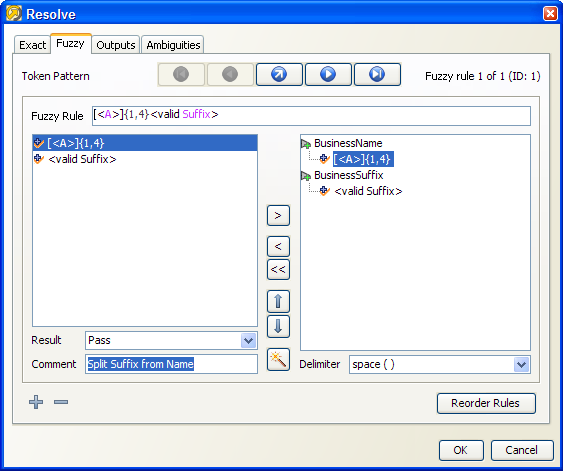
Description of the illustration ''exampleresolvefuzzyrule.png''
This then works as follows (drilling down on the rule in the Resolution Rule view):
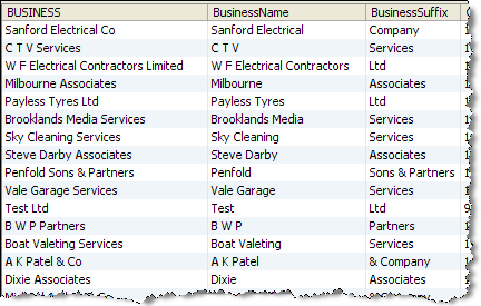
Description of the illustration ''exampleresolvefuzzyresults.png''
Note on the effect on resolution rules of deleting input or output attributes:
The deletion of input or output attributes from the Parse processor will affect any resolution rules that use those attributes.
If you delete an output attribute, it is also deleted from any Exact or Fuzzy resolution rules. The rules themselves, however, are not deleted. This is in order to preserve an attempt to resolve records according to your preferences, and not delete any mappings to other attributes that might still be valid.
In extreme cases, this can lead to resolution rules that are 'empty', as they only contained token mappings to attributes that no longer exist. More commonly, it will lead to rules that leave some data unmapped.
If you delete an input attribute, this naturally affects the token patterns that are generated in the data, and therefore makes it less likely that your resolution rules are valid.
In general, you should aim to begin creating and modifying resolution rules when all classifications and reclassifications are complete. Output attributes should normally be added (or perhaps renamed), but rarely deleted once they are used within resolution rules.
Automatic extraction is an optional feature, used to create useful output from parsing without the need to use any specific resolution rules. It is also useful to use it in conjunction with exact and/or fuzzy resolution rules, to create the best possible output for the remaining patterns (that do not match any specific rules). The aim of automatic extraction is to reflect the various token classifications of the input data directly in the output of the Parse processor.
When used, output attributes are automatically created for each distinct token classification tag used in the Classify and Reclassify stages. Tokens that match any of these tags are automatically extracted from each token pattern to these output attributes. Where a pattern contains multiple tokens with the same tag (for example, <valid Forename><valid Forename>...), these are all mapped to the same output attribute, separated using the delimiter that you choose (comma by default).
An additional output attribute is also created (Parse.UnclassifiedData). All tokens that are not specifically classified using a classification or reclassification rule are extracted to this attribute, again separated using the delimiter that you choose.
Automatic extraction can be enabled or disabled from the Outputs tab of the Resolve sub-processor. The delimiter placed between tokens, when more than one token in a given record is classified with the same tag, can also be changed.
Example of Automatic Extraction
By default; that is, without any exact or fuzzy resolution rules, automatic extraction will map (for a Parse processor checking and separating data in a NAME attribute) all classified tokens to output attributes of the same name, and mapping all remaining unclassified tokens to Parse.UnclassifiedData.
When drilling down to see the output data from the Parse processor, it is useful to use the Show Flags toggle on the Results Browser to see all the flag attributes the parser adds, including the selected token pattern, and the assigned Result and Comment.
1.3.9.11 Select
Select is a sub-processor of Parse. The Select step takes all of the possible generated token patterns describing each record and attempts to select the pattern that corresponds to its best understanding of the data, using a combination of criteria.
The criteria used are:
-
The number of tokens that are unclassified
-
The frequency of occurrence of each possible description across the data set (optional)
-
The confidence level of the classifications (valid or possible)
Selection uses a tunable algorithm to select the token pattern that best describes the data. There are times when a single token pattern cannot be selected - such as because two or more candidate patterns have the same number of unclassified tokens, occur a similar number of times across the data set, and have the same confidence levels in their classifications. In this case, the record is marked as having an ambiguity in its pattern selection. Where a record has one or more ambiguities in its selection, it can be assigned a Result (according to the option for Ambiguous Patterns in the Resolve step), but its data cannot be mapped to an output format.
The Parse processor performs selection in order to gain the best understanding of the tokens in each input record, which is then used in the Resolve step to give a result, and to resolve the data into a new output format.
For example, when parsing a single NAME field, the data "ADAM SCOTT" might be understood by simple classification rules to be either "<valid Forename>_<valid Surname>" or "<valid Surname>_<valid Forename>". The correct answer probably depends on the expected format of the data in the data set. If most of the remaining names are in the format "<Forename> <Surname>", then that seems the most likely pattern, and the person's name is most likely to be Adam Scott. However, if the remaining names are normally in the format "<Surname> <Forename>", then it is more likely that the person's name is Scott Adam.
Also, if a token has been classified with two different token checks, and with two different confidence levels, for example, if the token "ADAM" has been designated as a <valid Forename> and as a <possible Surname>, then by implication, it is more likely to be a <valid Forename>.
To understand how to configure the Select sub-processor, it is important to understand the logic used for selecting the best pattern.
This option defines the treatment of delimiter tokens by the selection process. In versions of EDQ prior to 8.1, delimiters were counted as unclassified tokens in the selection process. By default, new processors created in later versions of EDQ do not include delimiters in the unclassified tokens count.
Since only the patterns with the fewest unclassified tokens will be passed through to the final selection algorithm, the delimiter classification can alter the behavior of the processor.
Discounting patterns with more unclassified tokens
Selection automatically discounts any patterns with more unclassified tokens than others. For example, when parsing addresses, the data "Newcastle Upon Tyne" in a Town attribute might generate the following token patterns, assuming both "Newcastle" and "Newcastle Upon Tyne" are in a list of valid Towns, and were therefore classified as <valid Town> tokens:
For example, when parsing addresses, the data "Newcastle Upon Tyne" in a Town attribute might generate the following token patterns, assuming both "Newcastle" and "Newcastle Upon Tyne" are in a list of valid Towns, and were therefore classified as <valid Town> tokens:
<valid Town>_<A>_<A>
<valid Town>
In this case, Parse will always prefer the second pattern, as it contains fewer unclassified tokens.
Select then attempts to select the best token pattern for a given record, using the following algorithm. The algorithm is tunable at certain points - as marked below - so that you can tune the sensitivity of selection.
The tunable parameters may all be adjusted in the Advanced tab.
| Step | Optional | Criterion Used | Logic | Tunable Parameters |
|---|---|---|---|---|
| 1 | Yes (See below) | Frequency of token pattern occurrence across sample data (generated from results) | a) Select the most frequent pattern if it is more frequent than any other possible pattern by n % (configurable).
If >1 possible pattern remains, proceed to b. b) Discount any patterns that are p % (configurable) less frequent than the most frequent pattern If >1 possible pattern remains, proceed to Step 2. |
n (defaults to 10%)
p (defaults to 20%) |
| 2 | No | Confidence level of token classifications in pattern (valid or possible) | Give each possible pattern a score as follows:
Starting with 100 points: a) Subtract q points for each unclassified token b) Subtract r points for each token with a confidence level of Possible. Then, select the highest scoring pattern if it is highest by s points. |
q (defaults to 10)
r (defaults to 5) s (defaults to 5) |
Selecting pattern using frequency sample (Step 1 in the table above)
This is an optional step, but is recommended for any complex parsing needs.
On the first run of the Parse processor, it is not possible to select the best token pattern by analyzing its frequency across the data set. This is because Parse first needs to generate all the possible patterns.
Once the Parse processor has run at least once:
-
You can create a new Pattern frequency sample from the latest results (data in the Reclassification View), by clicking on the + button.
-
You can update a selected Pattern frequency sample from the latest results, by clicking the ^ button.
Using a static sample, rather than automatically using the pre-selection patterns data generated on each run, ensures predictable selection for the Parse processor, regardless of the size of the input data set. This ensures that provided the sample is the same, the same description will always be selected for a given record.
Updating the Results is often necessary, since you may iterate round many runs of the parser, and changes of classification and reclassification rules, before generating a set of descriptions that you are happy with.
Options are available to tune the parameters used in the pattern selection algorithm described in the section above. These options should only be changed by advanced users who are aware that changing them may have significant effects on the 'intelligence' of the parser.
Note that in this example, all the tunable parameters of the selection algorithm use their default values (as above).
In the analysis of a single NAME attribute, a record with the value "DR Adam FOTHERGILL ESQ" might produce the following potential token patterns (amongst others):
1. <valid Title>_<possible Surname>_<possible Surname>_<valid Honorific>

2. <valid Title>_<valid Forename>_<possible Surname>_<valid Honorific>

3. <valid Title>_<valid Forename>_<possible Surname>_<possible Surname>

4. <A>_<A>_<A>_<A>
Etc.
First of all, pattern 4 will be discounted, as it contains more unclassified tokens than any of the other patterns.
The remaining 3 token patterns are then passed to the selection algorithm:
At step 1a, if one of the patterns is more than 10% more frequent than either of the others in the sample data, this pattern will be selected. If not, the logic would proceed to step 1b.
At step 1b, if any of the patterns are more than 20% less frequent in the sample data than the most common pattern, these patterns would be discounted. If more than one pattern remained, the logic would proceed to step 2.
At step 2, the remaining patterns would be scored. Assuming patterns 1, 2 and 3 were all to remain, they would be scored as follows:
Pattern 1: 100 points – 10 points for 2 Possible tokens  = 90 points
Pattern 2: 100 points – 5 points for 1 Possible token = 95 points
Pattern 3: 100 points – 10 points for 2 Possible tokens  = 90 points
So, in this case pattern 2 would be selected, assuming the default threshold difference of 5 points (and not a higher value) is used.
Once you are happy with the way token patterns are selected, the final step in configuring a Parse processor is to Resolve data.
1.3.9.12 Tokenize
Tokenize is a sub-processor of Parse. The Tokenize sub-processor performs the first step of parsing by breaking up the data syntactically into an initial set of Base Tokens, by analyzing the characters, and sequences of characters, in the data.
Note that in the context of parsing, a Token is any 'unit' of data, as understood by the Parse processor. The Tokenize step forms the first set of Tokens - termed Base Tokens. Base Tokens are typically sequences of the same type of character (such as letters or numbers) separated by other types of character (such as punctuation or whitespace). For example, if the following data is input
| Address1 |
|---|
| 10 Harwood Road |
| 3Lewis Drive |
then the Tokenize step would break up the data into the following Base Tokens, using its default rules:
| Address1 | Base Tokens | Pattern of Base Tokens |
|---|---|---|
| 10 Harwood Road | "10" - tagged 'N' to indicate a number
" " - tagged '_' to indicate whitespace "Harwood" - tagged 'A' to indicate a word " " - tagged '_' to indicate whitespace "Road" - tagged 'A' to indicate a word |
N_A_A |
| 3Lewis Drive | "3" - tagged 'N' to indicate a number
"Lewis" - tagged 'A' to indicate a word " " - tagged '_' to indicate whitespace "Drive" - tagged 'A' to indicate a word |
NA_A |
However, you may want to ignore certain Base Tokens in further analysis of the data. For example, you may not want to classify the whitespace characters above, and may want to ignore them when matching resolution rules. It is possible to do this by specifying the characters you want to ignore as of a WHITESPACE or DELIMITER type in the Base Tokenization Reference Data. See Configuration below.
Use Tokenize to gain an initial understanding of the contents of the data attributes that you want to Parse, and to drive the way the data is understood. Normally, you can use the default set of tokenization rules to gain this understanding, and then refine them if needed - for example because a specific character has a specific meaning in your data and you want to tag it differently from other characters. Often, the default tokenization rules will not need to be changed.
The tokenization rules consist of the following Options:
| Option | Type | Purpose | Default Value |
|---|---|---|---|
| Character Map | Character Token Map | Maps characters (by Unicode reference) to a character tag, a grouped character tag, and a character type.
See Note below. |
*Base Tokenization Map |
| Split lower case to upper case | Yes/No | Splits sequences of letters where there is a change from lower case to upper case into separate tokens (for example, to split "HarwoodRoad" into two base tokens - "Harwood" and "Road"). | Yes |
| Split upper case to lower case | Yes/No | Splits sequences of letters where there is a change from upper case to lower case into separate tokens (for example, to split "SMITHjohn" into two base tokens - "SMITH" and "john"). | No |
Note on the Character Map Reference Data
The Reference Data used to tokenize data is of a specific format, and is important to the way Tokenize works.
The following screenshot of the default Reference Data explains the purpose of each column. The columns are described below.
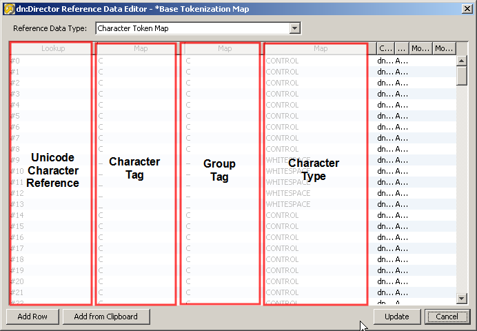
Description of the illustration ''basetokenizationmap.png''
Unicode character reference: The Unicode character reference is used by Tokenize in order to identify the character that will be mapped to a given character tag in the first step of tokenization. For example, the character reference #32, representing the Space character, is mapped to a character tag of '_' by default.
Note:
The default *Base Tokenization map is designed for use with Latin-1 encoded data, as are the alternative *Unicode Base Tokenization and *Unicode Character Pattern maps. If these maps are not suited to the character-encoding of the data, it is possible to create and use a new one to take account of, for example, multi-byte Unicode (hexadecimal) character references.Character tag: The Character tag is used in the first step of tokenization to assign each character in the data (identified by Unicode character reference) a given tag - for example all lower case letters might be assigned a character tag of 'a'.
Group tag: The Group tag is used in the second step of tokenization to group sequences of character tags with the same Group tag. Sequences of character tags with the same group tag, and the same character type, will be grouped to form a single token.For example, the first phase of tokenization might tag the data "103" as "NNN", using character tags, but as there are three characters with the same group tag ('N') and the same character type (NUMERIC), in sequence, these are grouped to form a single Base Token ("103"), with a Base Token Tag of 'N'.
Note that the behavior for ALPHA characters is slightly different, as the user can choose whether or not to split tokens where there is a sequence of lower case and upper case letters. By default, tokens are split on transition from lower case to upper case, but not from upper case to lower case. For example, the data "Michael" has the sequence of character tags 'Aaaaaaa', but has a transition in character type from ALPHA_UPPERCASE to ALPHA_LOWERCASE after the first letter. If the user keeps the default setting of the Split Upper to Lower Case option as not set, this will be grouped to form a single Base Token ("Michael") with a Base Token tag of 'A', as the character tags 'a' and 'A' both share the same group tag, and because the user is not splitting data on the transition of character type.
Character type: The Character type is used to split up data. In general, a change of character type causes a split into separate base tokens. For example, the string 'deluxe25ml' will be split into three base tokens - 'deluxe', '25' and 'ml'. These three base tokens will then be tagged according to their character and group tags. The exception to this rule is that, by default, a change of character type from ALPHA_UPPERCASE to ALPHA_LOWERCASE does not cause a split in tokens. This is in order to preserve tokens that are in proper case - for example, not to split 'Michael' into two tokens ('M' and 'ichael').
The user can change this behavior by selecting the option to Split Upper to Lower case.
The user can also choose to keep all strings of alpha characters together by de-selecting the option to Split Lower to Upper case. This would have the effect of keeping 'DelUXE' as one token.
Also, certain characters may be marked with a type of either WHITESPACE or DELIMITER. These characters can be ignored in later rules for matching sequences of tokens. For example, in Reclassify or Resolve, if you want to match a pattern of <Token A> followed by <Token B>, you may not care whether or not there are whitespace or delimiter characters in between them. The possible character types are NUMERIC, CONTROL, PUNCTUATION, SYMBOL, ALPHA_UPPERCASE, ALPHA_LOWERCASE and UNDEFINED.
Note also that the Comment column in the Reference Data explains the actual character to which the Unicode Character Reference refers - for example to tell you that #32 is the Space character etc.
Using different rules for different input attributes
By default, the same tokenization rules are applied to all the attributes input to the Parse processor. Normally, attribute-specific tokenization rules will not be required. However, you can change this by selecting an attribute on the left-hand side of the pane, and selecting the option to Enable attribute-specific settings. This may be required if you are analyzing many attributes with different characters as significant separators.
When specifying attribute-specific rules, it is possible to copy the settings for one attribute to another, or to reapply the default 'Global' settings using the Copy From option.
In this example, the default rules are used to tokenize some address data, with the following results:
(Note that in this case leading and trailing whitespace was trimmed from each attribute before parsing using the Trim Whitespace processor.)
The following table shows a summary of each distinct pattern of Base Tokens across all input attributes.
| ADDRESS1.trimmed | ADDRESS2.trimmed | ADDRESS3.trimmed | POSTCODE.trimmed | Count | % |
|---|---|---|---|---|---|
| <A>_<A><,> | <A> | <A><N>_<N><A> | 119 | 5.9 | |
| <A>_<A><,>_<A>_<A> | <A> | <A><N>_<N><A> | 95 | 4.7 | |
| <A>_<A><,> | <A> | <A> | <A><N>_<N><A> | 73 | 3.6 |
| <A>_<A><,>_<A>_<A> | <A> | <A> | <A><N>_<N><A> | 58 | 2.9 |
| <N>_<A>_<A><,> | <A> | <A><N>_<N><A> | 55 | 2.7 | |
| <A>_<A><,>_<A> | <A> | <A><N>_<N><A> | 49 | 2.4 | |
| <A>_<A><,> | <A> | <A><N>_<N><A> | <A><N>_<N><A> | 40 | 2.0 |
| <N>_<A>_<A><,> | <A> | <A> | <A><N>_<N><A> | 35 | 1.7 |
The following table shows a drilldown on the top Base Token pattern:
| ADDRESS1.trimmed | ADDRESS2.trimmed | ADDRESS3.trimmed | POSTCODE.trimmed |
|---|---|---|---|
| Tempsford Hall, | Sandy | SG19 2DB | |
| West Thurrock, | Purfleet | RM19 1PA | |
| Hayes Lane, | Stourbridge | DY9 8PA | |
| Middleton Road, | Oswestry | SY11 2RB | |
| Freshwater Road, | Dagenham | RM8 1RU | |
| College Road, | Birmingham | B8 3TE | |
| Ranelagh Gdns, | London | SW6 3PR | |
| Trumpington Road, | Cambridge, | CB2 2AG |
The next step in configuring a Parse processor is to Classify data.
1.3.9.13 Unicode Character Reference
The Unicode character reference is used by Tokenize in order to identify the character that will be mapped to a given character tag in the first step of tokenization. For example, the character reference #32, representing the Space character, is mapped to a character tag of '_' by default.
Note:
The default *Base Tokenization map is designed for use with Latin-1 encoded data, as are the alternative *Unicode Base Tokenization and *Unicode Character Pattern maps. If these maps are not suited to the character-encoding of the data, it is possible to create and use a new one to take account of, for example, multi-byte Unicode (hexadecimal) character references.1.3.9.14 Using Attribute Tags
The Map subprocessor of the Parse processor defines internal attributes for the Parse processor and maps the actual input attributes to them. The rest of the Parse processor's functionality is defined in terms of the internal attributes, so configured Parse processors can be re-used with a variety of input data sources simply by remapping the inputs. Each internal attribute is identified by a name, which is defined by the user who configures the Parse processor, and an attribute tag, which is automatically generated and cannot be edited. Attribute tags take the form a1, a2, a3 and so on.
Attribute tags can be used to distinguish between instances of the same token which originated from different input attributes. For example, a Parse processor which is being used to analyze name data may define three internal attributes: Title, Forename and Surname. By using attribute tags, a valid title which was extracted from the 'Title' field can be treated differently from a valid title which was extracted from a 'Forename' field, and so on.
This distinction is made in the Resolve subprocessor. If we consider just one possible token pattern:
<valid Title> <valid Forename> <valid Surname>
we can immediately see that it includes no reference to which attributes each token was contained in at the input stage. Without the use of attribute tags, any of the following four input patterns will be resolved the same way:
Table 1-124 Resolution of Input Patterns
| Pattern | Title (a1) | Forename (a2) | Surname (a3) |
|---|---|---|---|
|
1 |
<valid Title> |
<valid Forename> |
<valid Surname> |
|
2 |
<valid Title> <valid Forename> |
<valid Surname> |
|
|
3 |
<valid Title> <valid Forename> <valid Surname> |
||
|
4 |
<valid Title> |
<valid Forename> <valid Surname> |
Records which contain correct data, correctly fielded are generally considered to be of higher quality than records which contain correct data which has been incorrectly fielded. On this basis, we can define a resolution rule for the first pattern which distinguishes it from the other patterns, simply by including the attribute tags in the search criteria. The search term specific to pattern 1 would be:
<valid a1.Title> <valid a2.Forename> <valid a3.Surname>
Including the non-specific search term in a subsequent resolution rule would catch patterns 2, 3 and 4, which could be assigned a different resolution result based on the lower quality of their formatting.
Note:
Because resolution rules are applied in order, the more specific rules must be tested for before the more generic rules. Otherwise, the generic rule will act on all the patterns without the specific match ever being considered.The following table gives further examples of search strings for resolution rules, and specifies which of the above patterns will match them:
Table 1-125 Further Examples of Search Strings
| Search string | Matching patterns |
|---|---|
|
<valid a1.Title> <valid a2.Forename> <valid a3.Surname> |
1 |
|
<valid Title> <valid a2.Forename> <valid a3.Surname> |
1, 2 |
|
<valid Title> <valid a2.Forename> <valid Surname> |
1, 2, 3 |
|
<valid Title> <valid Forename> <valid a3.Surname> |
1, 2, 4 |
1.3.10 Third-party Processors
Third party processors use integrations with third party products to perform data analysis and transformation. Third party processors are normally enabled when EDQ detects a valid installation of the third party software required by the processor.
1.3.10.1 Address Verification
The Address Verification processor (AV) is used to verify and standardize address data from any country. It also provides geocoding.
Note:
If the processor has not been correctly installed it will still run but all the output fields will be left blank, except for Accuracy Code, which will have a value of -1.0.Use the Address Verification processor:
-
to standardize addresses to a format;
-
to check whether an address is correct;
-
to complete partial addresses; and
-
to enhance address data with geocodes.
This processor always appears with a re-run marker, indicating that it will be completely re-executed each time the process is run, regardless of whether or not its configuration has changed. This will also mean that processors that are downstream of the processor will need to be rerun. This is because there may be changes made outside of the EDQ application that could lead to different results on subsequent executions.
The Input attribute mappings are used as clues by the processor as to which Input attributes may contain specific data types, according to the initial structure of the address data. It is not normally necessary to parse addresses fully into all the different Input attributes before putting data through Address Verification. In many cases, it is sufficient to simply add address data to the Input address lines (as long as a country is provided), as the Address Verification processor itself will internally parse addresses before matching them against country-specific reference data. However, if addresses are well structured, more effective verification results may be seen if the corresponding input attribute mappings are used (for example, if an Input attribute normally contains postal codes, it is best to map it to the Postal Code input attribute rather than simply mapping it in as an address line.)
-
Organization
-
Up to 8 address line values
-
Double Dependent Locality
-
Dependent Locality
-
Locality
-
Administrative Area
-
Postal Code
-
Country
-
Postal Box
-
Sub Building
-
Building
-
Premise
-
Thoroughfare
-
Dependent thoroughfare
-
Super Administrative Area
-
Sub Administrative Area
Note:
The Country input must be populated with a country name or code. Without it, Address Verification cannot verify an address or produce an Accuracy Code.| Option | Description | Settings |
|---|---|---|
| Processing mode | Whether to verify the input address or search all installed data and return multiple results. | Verify (Best Match): 1 to 1 - Checks the reference data and returns the best match.
Verify (Allow Multiple Results): Attempts to verify the input address 1 to 1, but allows Address Verification to return multiple possible results if the input address has an Ambiguous verification result. Search: 1 to Many - Checks the reference data and returns multiple matches. Allows searching across countries, for example. |
| Maximum number of results | An optional upper limit on number of results that can be returned.
Note: This field is greyed out if Verify (Best Match) is selected. |
Numeric field, maximum of 15 characters. |
| Geocode | Whether matching geocodes are to be returned. | Yes
No |
| Output address separator | The symbol used to separate the address elements. | Selection of punctuation symbols and special characters. |
| Output script | The output is converted into the script selected. | Drop-down list of available scripts. Native - the default - returns the output in its original script. |
| Output Casing | The case the output is returned in. | The available options are Title (default - the first character of each word is upper case, the others are lower case), Upper or Lower. |
| Additional options | Free-text field. | There are additional options available that are not listed on the Address Verification: Options tab.
To use these options, enter them and the specified value in this free-text field. For example:
Note:
|
The following table lists all the possible AV output fields. The exact output for each set of data depends on the settings of the AV processor, the original address data, and the information available for the country.
Note:
The CASS, AMAS and SERP options will only work if the appropriate additional Loqate libraries and data are installed.| Output Field | Description |
|---|---|
| av.Address | The full address, matched/verified and correctly formatted for mailing in the relevant country. |
| av.CountryName | The full country name. |
| av.ISO3166-2 | The ISO3166 two-character country code. |
| av.ISO3166-3 | The ISO3166 three-character country code. |
| av.ISO3166-N | The ISO3166 three-digit numeric country code. |
| av.SuperAdministrativeArea | The largest geographic data element within a country. |
| av.AdministrativeArea | The most common geographic data element within a country; e.g. a US state or Canadian Province. |
| av.SubAdministrativeArea | The smallest geographic data element; e.g. a US county. |
| av.Locality | The most common population center data element in a country; e.g. a city or municipality. |
| av.DependentLocality | A smaller population center data element; e.g. a Turkish neighborhood. |
| av.DoubleDependentLocality | The smallest population center data element, depending on the contents of the Locality and DependentLocality fields; e.g. a UK village. |
| av.Thoroughfare | The most common street or block data element within a country; e.g. a street. |
| av.ThoroughfarePreDirection | The prefix direction contained within the Thoroughfare field. E.g. if Thoroughfare contains "N MAIN ST" ThoroughfarePreDirection will contain "N". |
| av.ThoroughfareLeadingType | The leading thoroughfare type indicator within the Thoroughfare field. E.g. if Thoroughfare contains "RUE DE LA GARE" ThoroughfareLeadingType will contain "RUE". |
| av.ThoroughfareName | The name indicator within the Thoroughfare field. E.g. if Thoroughfare contains "N MAIN ST" ThoroughfareName will contain "MAIN". |
| av.ThoroughfareTrailingType | The trailing thoroughfare type indicator within the Thoroughfare field. E.g. if Thoroughfare contains "N MAIN ST" ThoroughfareTrailingType will contain "ST". |
| av.ThoroughfarePostDirection | The postfix directional contained within the Thoroughfare field. E.g. if Thoroughfare contains "MAIN ST N" ThoroughfarePostDirection will contain "N". |
| av.DependentThoroughfare | The dependent street or block data element within a country; e.g. UK Dependent Street. |
| av.DependentThoroughfarePreDirection | The prefix directional contained within the DependentThoroughfare field. E.g. if DependentThoroughfare contains "N MAIN ST" DependentThoroughfarePreDirection will contain "N". |
| av.DependentThoroughfareLeadingType | The leading thoroughfare type indicator within the DependentThoroughfare field. E.g. if DependentThoroughfare contains "RUE DE LA GARE" DependentThoroughfareLeadingType will contain "RUE". |
| av.DependentThoroughfareName | The name indicator within the DependentThoroughfare field. E.g. if DependentThoroughfare contains "N MAIN ST" DependentThoroughfareName will contain "MAIN". |
| av.DependentThoroughfareTrailingType | The trailing thoroughfare type indicator within the DependentThoroughfare field. For instance, if DependentThoroughfare contains "N MAIN ST" DependentThoroughfareTrailingType will contain "ST". |
| av.DependentThoroughfarePostDirection | The postfix directional contained within the DependentThoroughfare field. E.g. if DependentThoroughfare contains "MAIN ST N" DependentThoroughfarePostDirection will contain "N". |
| av.Building | The descriptive name identifying an individual location. |
| av.BuildingLeadingType | The leading building type indicator within the Building field. E.g. if Building contains "BLOC C" BuildingLeadingType will contain "BLOC". |
| av.BuildingName | The name indicator within the Building field. E.g. if Building contains "WESTMINSTER HOUSE" BuildingName will contain "WESTMINSTER". |
| av.BuildingTrailingType | The trailing building type indicator within the Building field. E.g. if Building contains "WESTMINSTER HOUSE" BuildingTrailingType will contain "HOUSE". |
| av.Premise | The alphanumeric code identifying an individual location. |
| av.PremiseType | The leading premise type indicator within the Premise field. E.g. if Premise contains "Plot 7/7A" PremiseType will contain "Plot". |
| av.PremiseNumber | The alphanumeric indicator within the Premise field. For instance, if Premise contains "Plot 7/7A" PremiseNumber contains "7/7A". |
| av.SubBuilding | The secondary identifiers for a particular delivery point, e.g. "FLAT 1" or "SUITE 212". |
| av.SubBuildingType | The leading sub-building type indicator within the SubBuilding field. E.g. if SubBuilding contains "FLAT 1" SubBuildingType will contain "FLAT". |
| av.SubBuildingNumber | The alphanumeric indicator within the SubBuilding field. E.g. if SubBuilding contains "FLAT 1" SubBuildingNumber will contain "1". |
| av.SubBuildingName | The descriptive name within the SubBuilding field. E.g. if SubBuilding contains "BASEMENT FLAT" SubBuildingName will contain "BASEMENT FLAT". |
| av.PostalCode | The complete postal code for a particular delivery point. |
| av.PostalCodePrimary | The primary postal code used for a particular country; e.g. USA Zip, Canadian Postcode or Indian PINcode. |
| av.PostalCodeSecondary | Secondary postal code information; e.g., USA Zip Plus 4. |
| av.Organization | The business name associated with a particular delivery point. |
| av.OrganizationName | The name indicator within the Organization field. E.g. if Organization contains 'Loqate Inc" OrganizationName will contain "Loqate", if a sufficient level of parsing detail exists for the country. |
| av.OrganizationType | The trailing type indicator contained within the Organization field. E.g. if Organization contains "Loqate Inc" OrganizationType will contain "Inc", if a sufficient level of parsing detail exists for the country. |
| av.PostBox | The type indicator contained within the PostBox field. E.g. if PostBox contains "PO BOX 1234" PostBoxType will contain "PO BOX", if a sufficient level of parsing detail exists for the country. |
| av.PostBoxNumber | The alphanumeric indicator within the PostBox field. E.g. if PostBox contains "PO BOX 1234" PostBoxNumber will contain "1234", if a sufficient level of parsing detail exists for the country. |
| av.Latitude | The WGS 84 latitude in decimal degrees format. |
| av.Longitude | The WGS 84 longitude in decimal degrees format. |
| av.DeliveryAddress | The full address minus the Organization, Locality hierarchy, AdministrativeArea hierarchy and PostalCode hierarchy fields, correctly formatted for mailing in the relevant country, including line breaks specified using the AddressLineSeparator option. |
| av.Geodistance | The possible radius in meters of Geocoding results that have been calculated as the average of multiple points. |
| av.Contact | The contact name. |
| av.Function | The function or job title. |
| av.Department | Organizational department information. |
| av.Unmatched | Any words that could not be matched to a particular address component. |
| avverify.amas.DPID | Delivery Point Identifier: a unique 8-digit number which is assigned for every new address to the source address database |
| avverify.amas.FloorType | Type of floor or level |
| avverify.amas.FloorNumber | Floor or level number (which can include alpha characters) |
| avverify.amas.LotNumber | Allotment number |
| avverify.amas.PostBoxNum | Postal delivery number if the address is a postal delivery type |
| avverify.amas.PostBoxNumberPrefix | Postal delivery number prefix related to the postal delivery number |
| avverify.amas.PostBoxNumberSuffix | Postal delivery number suffix related to the postal delivery number |
| avverify.amas.PrimaryPremise | Thoroughfare number for a property (first number in a property ranged address) |
| avverify.amas.PrimaryPremiseSuffix | Suffix for the thoroughfare number |
| avverify.amas.SecondaryPremise | Second thoroughfare number (only used if the property has a ranged address. For example, 23-25) |
| avverify.amas.SecondaryPremiseSuffix | Suffix for the second thoroughfare number |
| avverify.amas.PreSortZone | Also known as Barcode Sort Plan (BSP) number. One of 54 individual sort regions around Australia. To qualify for Australia Post's PreSort Letters Service, letters must be sorted based on this number. |
| avverify.amas.PrintPostZone | Also known as a PreSort Indicator. To qualify for Australia Post's Print Post Service, letters must be sorted based on this number. |
| avverify.amas.Barcode | Barcode based on the DPID |
| avverify.amas.PrimaryAddressLine | Primary address line in standardized format |
| avverify.amas.SecondaryAddressLine | Secondary address line in standardized format |
| avverify.cass.AutoZoneIndicator | Automated Zone Indicator, where
|
| avverify.cass.CarrierRoute | Carrier route code assigned to a mail delivery or collection route within a 5-digit ZIP Code, also referred to as CRID. There are 5 types:
|
| avverify.cass.CMRAIndicator | Indicates whether the address is associated with a Commercial Mail Receiving Agency(CMRA).
|
| avverify.cass.CongressionalDistrict | The congressional district to which the address belongs |
| avverify.cass.DefaultFlag | A value of "Y" indicates that the record matched to a high rise default, rural route default, or street default record in the ZIP+4 file. |
| avverify.cass.DeliveryPointBarCode | 3-digit code which consists of the 2-digit delivery point code and 1-digit check digit.This is used to create the 12-digit POSTNET barcode which consists of the 5-digit ZIP Code, 4-digit ZIP+4 addon code, and this 3-digit code. |
| avverify.cass.DPVConfirmedIndicator | Indicates the deliverability of the address using one of the following values:
|
| avverify.cass.DPVFootnotes | Delivery Point Validation footnotes. This field is used with the DPVConfirmedIndicator field determine the input address' validity and deliverability.
|
| avverify.cass.eLOTCode | eLOT directional indicator. See the eLOTNumber field for additional information. Values:
|
| avverify.cass.eLOTNumber | A 4-digit sequence number for eLOT (Enhanced Line of Travel). This number combined with the eLOTCode field is used in mail sorting. eLOT processing may be used by mailers to qualify for enhanced carrier route presort discounts. |
| avverify.cass.EWSFlag | A value of "Y" indicates that the address matched a record in the EWS (Early Warning System) file, thus resulting in a ZIP+4 no match |
| avverify.cass.FalsePositiveIndicator | The False Positive table flags the False Positive addresses. This flag determines whether a mailing list is being generated or created during validation. The USPS does not allow creating a mailing list through DPV certification.
|
| avverify.cass.FIPSCountyCode | A 5-digit FIPS (Federal Information Processing Standard) code which uniquely identifies counties. |
| avverify.cass.Footnotes | Footnote string
|
| avverify.cass.LACSLinkCode | Code returned by LACSLink after querying the LACSLink database.
|
| avverify.cass.LACSLinkIndicator | Indicator returned by LACSLink after querying the LACSLink database.
|
| avverify.cass.LACSStatus | A value of "L" indicates that the input address matched an entry in the Locatable Address Conversion Service database and the input address has been converted from a rural-style address to a city-style address. |
| avverify.cass.NoStatIndicator | Indicates the address is not receiving delivery, and the address is not counted as a possible delivery. These addresses are not receiving delivery because 1) delivery has not been established; 2) customer receives mail as a part of a drop; or 3) the address is no longer a possible delivery because the carrier destroys or returns all of the mail.
|
| avverify.cass.PMBNumber | Parsed PMB number following the PMB designator |
| avverify.cass.PMBType | Parsed Private Mailbox (PMB) designator |
| avverify.cass.PrimaryAddressLine | Primary delivery address line. This can include any of the following:
|
| avverify.cass.RecordType | Record type of address that is confirmed as a valid delivery address. Values:
|
| avverify.cass.ReturnCode |
|
| avverify.cass.ResidentialDelivery | This field indicates whether the input address is a residential address or a business address. Values:
Note: This field is only available if RDI data pack is installed together with CASS. |
| avverify.cass.SecondaryAddressLine | Secondary delivery address line (if present). |
| avverify.cass.SUITELinkFootnote | Code returned by SuiteLink after querying the SuiteLink database. Values:
|
| avverify.cass.VacantIndicator | Indicates that the delivery point was active in the past, but is currently vacant (in most cases, unoccupied over 90 days) and is not receiving deliveries. Values:
|
| avverify.serp.SerpStatusEx | V (Valid)
C (Correctable): Correctable fields will have been corrected to their right values in the output. N (Invalid) |
| avverify.serp.Questionable | QR (for "Questionable-Rural")
QU (for "Questionable-Urban") Empty - the address is not questionable. |
| avverify.serp.DeliveryInstallationAreaName | Station/Postal Installation Area Name |
| avverify.serp.DeliveryInstallationType | Station/Postal Installation/Outlet Type |
| avverify.serp.DeliveryInstallationQualifierName | Name of the Postal Installation |
| avverify.serp.RouteType | The type of a Route Address: Rural Route, Military Route etc. |
| avverify.serp.RouteNumber | Identifies Route Number for a Route Address |
| avverify.serp.AdditionalContentType | Contains Site Or Compartment Specifier |
| avverify.serp.AdditionalContentNumber | Contains Site or Compartment Number |
| Flag Name | Details |
|---|---|
| av.AccuracyCode | A code that indicates how accurately each address has been identified and matched.
Note: For the multiple output options (Verify: Allow Multiple Results and Search), an Accuracy Code is returned for each result found. |
| av.ResultCount | Number of addresses returned. Always "1" for Verify mode. |
| av.MatchScore | The match between the input and the closest reference match, expressed as a percentage. This is extracted from the Accuracy code. |
| av.GeoAccuracy | A code that indicates whether one or more Geocodes associated with the address have been identified. |
Note:
If the Returned field status flag? option on the Options tab of the processor is set to Yes, an additional flag will generated for each output attribute, with a numeric value indicating the verification status of each one.| Code | Description |
|---|---|
| 0 | Not Applicable: Field is not applicable to return field status. |
| 1 | Verified No Change: Field has been verified using relevant reference data, no changes were needed. |
| 2 | Verified Alias Change: Field has been verified using relevant reference data, an alias change was made during parsing (see 7: Identified Alias). |
| 3 | Verified Small Change: Field has been verified using relevant reference data, a small spelling change was made. |
| 4 | Verified Large Change: Field has been verified using relevant reference data, a large spelling change was made. |
| 5 | Added: Field has been added using relevant reference data. |
| 6 | Identified No Change: Field has been identified using relevant lexicon data, no changes were needed. e.g. an input value of "PO Box 1234" may be identifiable as a PostBox, but if it is unable to be verified then status 6 will be returned. |
| 7 | Identified Alias: Field has been identified using relevant lexicon data, an alias change was made. e.g. an input value of 'Avnue' may be identifiable as an alias to the ThoroughfareType 'Ave'. |
| 8 | Identified Context: Field has been identified using relevant context rules. e.g. an input Address of "123 sdovnsdv San Bruno CA USA" may identify the word "sdovnsdv" as a Thoroughfare, but only because of the context in which it appears (after an identifiable Premise Number, and before an identifiable Locality). |
| 9 | Empty: Field is empty. |
| 10 | Unrecognized: Field is unrecognized. |
This code consists of the following components:
Description of the illustration ''OAV_address_code.png''
A. Verification status - The level of verification.
-
V: Verified - A complete match was made between the input data and a single record from the available reference data.
-
P: Partially verified - A partial match was made between the input data and a single record from the available reference data.
-
U: Unverified - Unable to verify. The output fields will contain the input data.
-
A: Ambiguous - More than one close reference data match.
-
C: Conflict - More than one close reference data match with conflicting values.
-
R: Reverted - Record could not be verified to the specified minimum acceptable level. The output fields will contain the input data.
B. Post-processed verification match level - The extent to which the input data matches the available reference data following the verification process.
-
5: Delivery Point (PostBox or SubBuilding).
-
4: Premise (Premise or Building).
-
3: Thoroughfare.
-
2: Locality.
-
1: Administrative Area.
-
0: None.
C. Pre-processed verification match level - The extent to which the input data matches the available reference data prior to the verification process.
-
5: Delivery Point (PostBox or SubBuilding).
-
4: Premise (Premise or Building).
-
3: Thoroughfare.
-
2: Locality.
-
1: Administrative Area.
-
0: None.
D. Parsing status - Whether it has been possible to parse all the data.
-
I: Identified and Parsed - Input data has been able to be identified and placed into components
-
U: Unable to parse - Not all input data has been able to be identified and parsed.
E. Lexicon identification match level - The level to which the input data has a recognized form through pattern and lexicon matching.
-
5: Delivery Point (PostBox or SubBuilding).
-
4: Premise (Premise or Building).
-
3: Thoroughfare.
-
2: Locality.
-
1: Administrative Area.
-
0: None.
F. Context identification match level - The context identification match level gives the level to which the input data can be recognized based on the context in which it appears.
-
5: Delivery Point (PostBox or SubBuilding).
-
4: Premise (Premise or Building).
-
3: Thoroughfare.
-
2: Locality.
-
1: Administrative Area.
-
0: None.
G. Postcode status - The extent to which the postcode has been verified.
-
P8: PostalCodePrimary and PostalCodeSecondary verified.
-
P7: PostalCodePrimary verified, PostalCodeSecondary added or changed.
-
P6: PostalCodePrimary verified.
-
P5: PostalCodePrimary verified with small change.
-
P4: PostalCodePrimary verified with large change.
-
P3: PostalCodePrimary added.
-
P2: PostalCodePrimary identified by lexicon.
-
P1: PostalCodePrimary identified by context.
-
P0: PostalCodePrimary empty.
H. Matchscore - The similarity between the input data and closest reference data match as a percentage between 0 (no match) and 100 (perfect match).
Also known as the Geocode, this flag consists of two values:
| Value | Description | Settings |
|---|---|---|
| Geocoding Status | Indicates whether a Geocode for the address has been found. | P: Point - A single geocode was found matching the input address
I: Interpolated - A geocode was interpolated from the input address's location in a range A: Average Multiple - Candidate geocodes were found to match the input address, and an average of these was returned U: Unable to geocode - A geocode was not able to be generated for the input address |
| Geocoding Level | Indicates the geographical accuracy of the Geocode. | 5: Delivery Point (PostBox or SubBuilding)
4: Premise (Premise or Building) 3: Thoroughfare 2: Locality 1: Administrative Area 0: None |
| Execution Mode | Supported |
|---|---|
| Batch | Yes |
| Real-Time Monitoring | Yes |
| Real-Time Response | Yes |
The Address Verification processor presents no summary statistics on its processing.
In the Data view, each input attribute is shown with the output attributes to the right.
None.
1.3.10.2 Capscan Matchcode
The Capscan Matchcode processor uses an installation of the Capscan Matchcode API to verify and standardize addresses. EDQ supports any data sets that have been purchased for use with the Capscan Matchcode API.
Addresses are verified against reference data supplied by Capscan. To use the Capscan Matchcode processor, you must have a licensed installation of the Capscan Matchcode API.
Use Capscan Matchcode to:
-
Verify addresses
-
Correct errors and missing information in addresses
-
Using Capscan's Commercial and Names data, check that the organizations and individuals associated with your addresses are listed at those addresses in Capscan's reference data
The following table describes the configuration options:
| Configuration | Description |
|---|---|
| Inputs | Specify any number of input attributes containing address data.
Note that Capscan Matchcode will work best if the address attributes are input in logical order (for example, Address1, Address2, Town, County, Postcode for UK addresses). For some addresses, it may be useful to input less data (for example, Address1 and Postcode), especially if the address fields contain information that is unlikely to be in the national address files. |
| Options | Specify the following options:
|
| Outputs | Describes any data attribute or flag attribute outputs. |
|
Data Attributes |
There are the following data attributes:
|
|
Flags |
There are the following flags:
|
The Capscan Matchcode processor presents no summary statistics on its processing.
In the Data view, each input attribute is shown with the output attributes to the right.
None.
In this example, Capscan Matchcode is used to match UK addresses against Royal Mail's PAF (Postal Address File):
| Address1 | Address2 | Address3 | Address 4 | ZipCode | capscan.MatchScore | capscan.OutputStatus |
|---|---|---|---|---|---|---|
| 2 Thrornham Drive | NORWICH | NR7 8HX | 99 | V | ||
| KILCREGGAN | 15 Seafield Street | ELGIN | IV30 1QZ | 80 | V | |
| 24 Kirkham Road | Heald Green | CHEADLE | SK8 3DT | 100 | V | |
| Lynmar | Temple Road | SOUTHAMPTON | SO19 9FE | 99 | V | |
| 1 Longfield Crescent | ILKESTON | DE7 4DE | 99 | V | ||
| 9 Cornwalis Drive | SHIFNAL | TF11 8UB | 86 | V | ||
| 3 Doonview Wynd | Doonfoot | Ayr | KA7 4HY | 99 | V | |
| 12 Canons Gate | HARLOW | CM20 1QE | 99 | V |
1.3.10.3 Experian QAS
The Experian QAS processor uses an installation of the Experian QAS Batch API (formerly known as the QAS QuickAddress Batch API) to verify and standardize addresses. EDQ supports any data sets that have been purchased for use with the Experian QAS Batch API. Default configurations (layouts) are provided for specific countries. It is also possible to standardize data to a user-created address output.
Addresses are verified by matching them against reference data supplied by Experian QAS. The reference data used is from various sources dependent on the country. See the Experian QAS Country Information Guides for details.
Names may also be verified against data supplied by Experian QAS, where such a data set is available for a given country, for example by using the QAS GBN Names data.
To use the Experian QAS processor, you must have a licensed installation of the Experian QAS Batch API on your EDQ server.
Note:
You may need to configure some system settings on your EDQ server to ensure that the Experian QAS Batch API and EDQ work together correctly.This processor is compatible with Experian QAS Batch API version 6.1 and above.
Use the Experian QAS processor:
-
To standardize addresses to a given format, so that postal town and postcode are in specified attributes.
-
To check whether an address is correct, or if not, in what way the address is not correct (see the MatchCode meaning below).
-
To check whether a name is correct and up-to-date for a given address (where the QAS data set exists).
-
To enhance data to add further information available in data files from QAS, such as grid references.
The following table describes the configuration options:
| Configuration | Description |
|---|---|
| Inputs | Specify any number of attributes containing Name or Address data.
Note: When using the Experian QAS processor in ALL mode, to allow verification of address data from many countries, it is useful to input the name of the country of the address to the API to assist it in searching for the relevant country base. If you do not have the name of the country in your data, you can add it by enhancing the data using the address data, or an ISO Code. |
| Options | Specify the following options:
|
| Outputs | Describes any data attribute or flag attribute outputs. |
|
Data Attributes |
The output data attributes are dependent on the layout used as defined in the QAWORLD.ini file of the Experian QAS installation. All valid layouts will be selectable in the Options of the Experian QAS processor. |
|
Flags |
There are the following flags:
|
| Execution Mode | Supported |
|---|---|
| Batch | Yes |
| Real time Monitoring | Yes |
| Real time Response | Yes |
Note:
This processor always appears with a re-run marker, indicating that it will be completely re-executed each time the process is run, regardless of whether or not its configuration has changed. This will also mean that processors that are downstream of the processor will need to be rerun. This is because there may be changes made outside of the EDQ application that could lead to different results on subsequent executions.The Experian QAS processor presents no summary statistics on its processing.
In the Data view, each input attribute is shown with the output attributes to the right.
| MatchCode Meaning |
|---|
| The number of records where Experian QAS returned either of the following results:
R - Full address and postcode found Q - Full address found, but no postcode P - Partial address found with postcode O - Partial address found, but no postcode N - Multiple addresses found with postcode M - Multiple addresses found, but no postcode L - Postcode found, but no address could be derived K - No address or postcode could be derived D - Unidentified country C - Country not available B - Blank A - Unprocessed |
| Subsequent processors may be used to classify valid addresses. For example, the Logic Check processor could be used to pass those records where MatchSuccess >O (that is, P, Q or R), and where MatchConfidenceLevel = 9 |
None.
In this example, a number of UK addresses are checked using the Experian QAS Batch API against the GBR layout:
| Whole Address | qas.MatchCode | qas.MatchSuccess |
|---|---|---|
| Filling Station, Ilkley Road(A65), Burley in Wharfedale, North Yorkshire, LS29 7BT | R013701a2020024390000000000 | R |
| Orbis, Cathedral Gardens, Manchester, Lancashire, M4 3PG | R53340000020040001000000000 | R |
| Moor End Livery, Tempsford Hall,, Sandy, SG19 2BD | P91300000024020000000000000 | P |
| C T V Services, CTV House, Lichfield Road Industrial Estate, Tamworth, Staffordshire, B79 7TA | P91300000024020400000000000 | P |
| 195 Temple Way ,,Bristol,BS99 7HD | O9030000002406000000000000 | O |
1.3.10.3.1 Layout ALL
The default configuration provided by EDQ produces the following output data attributes:
| Attribute | Value |
|---|---|
| AddressLine1 | The matched Organization |
| AddressLine2 | The matched Post-Office Box |
| AddressLine3 | The matched initial Building or Street element |
| AddressLine4 | The matched final Building or Street element |
| AddressLine5 | The matched Village |
| AddressLine6 | The matched Town / City |
| AddressLine7 | The matched County / State / Province |
| AddressLine8 | The matched Postal Code |
| AddressLine9 | The matched 3 character Country Code |
The output data attributes are given generic names, such as AddressLine1, since generic values are used (in order to use mixed international data).
1.3.10.3.2 Layout DEU
The default configuration provided by EDQ produces the following output data attributes:
| Data Attribute | Value |
|---|---|
| qas.Organization | The matched Organization |
| qas.Department1 | The matched first Department |
| qas.Department2 | The matched second Department |
| qas.POBox | The matched PO Box Type |
| qas.Street | The matched Street |
| qas.BuildingNumber | The matched Building Number |
| qas.PostalCode | The matched Postal Code |
| qas.Town | The matched Town |
| qas.TownRegion | The matched Town-Region (used to distinguish between different towns that have the same official postal name) |
| qas.District | The matched District |
| qas.StateName | The matched State |
| qas.Country | The matched Country |
| qas.UnusedInput | An array containing all the address elements that were not matched by the API to a target address |
1.3.10.3.3 Layout_DNK
The default configuration provided by EDQ produces the following output data attributes:
| Data Attribute | Value |
|---|---|
| qas.BuildingNumber | The matched Building Number |
| qas.BuildingName | The matched Building Name |
| qas.Floor | The matched Floor * |
| qas.ApartmentNumber | The matched Apartment Number |
| qas.ApartmentName | The matched Apartment Name* |
| qas.Street | The matched Street |
| qas.PostalCode | The matched Postal Code |
| qas.PostalDistrict | The matched Postal District |
| qas.Town | The matched Town |
| qas.Country | The matched Country |
| qas.UnusedInput | An array containing all the address elements that were not matched by the API to a target address |
* See the QAS documentation for the meaning of the codes used here.
1.3.10.3.4 Layout ESP
The default configuration provided by EDQ produces the following output data attributes:
| Data Attribute | Value |
|---|---|
| qas.BuildingNumber | The matched Building Number |
| qas.Street | The matched Street |
| qas.PostalCode | The matched Postal Code |
| qas.Region | The matched Region |
| qas.Province | The matched Province |
| qas.Town | The matched Town |
| qas.UnusedInput | An array containing all the address elements that were not matched by the API to a target address |
1.3.10.3.5 Layout FRA
The default configuration provided by EDQ produces the following output data attributes:
| Data Attribute | Value |
|---|---|
| qas.CEDEXOrganisation | The matched CEDEX Organization |
| qas.CEDEXDepartment | The matched CEDEX Department |
| qas.POBoxType | The matched PO Box Type |
| qas.Location | The matched Location for example, Centre Commercial |
| qas.Number | The matched Building Number |
| qas.Street | The matched Street |
| qas.Locality | The matched Locality |
| qas.Postcode | The matched Postcode |
| qas.Town | The matched Town |
| qas.Departement | The matched Departement |
| qas.INSEECode | The matched INSEE Code (five character alpha-numeric code used to identify a locality) |
| qas.Country | The matched Country |
| qas.UnusedInput | An array containing all the address elements that were not matched by the API to a target address |
1.3.10.3.6 Layout GBR
The default configuration provided by EDQ produces the following output data attributes:
| Data Attribute | Value |
|---|---|
| qas.Organisation | The matched Organization |
| qas.POBox | The matched PO Box |
| qas.SubBuildingName | The matched Sub-building Name |
| qas.BuildingName | The matched Building Name |
| qas.BuildingNumber | The matched Building Number |
| qas.DependentThoroughfare | The matched Dependent Thoroughfare |
| qas.Thoroughfare | The matched Thoroughfare |
| qas.DoubleDependentLocality | The matched Double Dependent Locality |
| qas.DependentLocality | The matched Dependent Locality |
| qas.Town | The matched Town |
| qas.SubmittedPNRLocality | The matched Locality (commonly used to identify part of a large town or city) |
| qas.County | The matched County |
| qas.Postcode | The matched Postcode |
| qas.UnusedInput | An array containing all the address elements that were not matched by the API to a target address. |
1.3.10.3.7 Layout LUX
The default configuration provided by EDQ produces the following output data attributes:
| Data Attribute | Value |
|---|---|
| qas.BuildingNumber | The matched Building Number |
| qas.BuildingName | The matched Building Name |
| qas.Street | The matched Street |
| qas.PostalCode | The matched Postal Code |
| qas.POBoxNumber | The matched PO Box Number |
| qas.Locality | The matched Locality |
| qas.Country | The matched Country |
| qas.UnusedInput | An array containing all the address elements that were not matched by the API to a target address |
1.3.10.3.8 Layout_NLD
The default configuration provided by EDQ produces the following output data attributes:
| Data Attributes | Value |
|---|---|
| qas.Postbus | The matched Postbus (equivalent of PO Box) |
| qas.HouseNumber | The matched House Number |
| qas.Street | The matched Street |
| qas.TownCity | The Matched Town / City |
| qas.Province | The matched Province |
| qas.PostalCode | The matched Postal Code |
| qas.Country | The matched Country |
| qas.UnusedInput | An array containing all the address elements that were not matched by the API to a target address |
1.3.10.3.9 Advanced Experian QAS API Configuration
The following features are intended for use by advanced users of Experian QAS or EDQ administrators only. These features involve editing the QAWorld.ini configuration file which is part of the QAS installation, and require some familiarity with customizing the Experian QAS Batch API.
Note that the EDQ application service must be restarted on the server for these changes to take effect.
It is possible to create your own layout for use by the Experian QAS Batch API, for example to use the API with newly purchased data sets from Experian QAS, or to change the format in which addresses are returned by the API. The easiest method is to copy an existing layout found in the QAWorld.ini file and to edit the copy. Ensure the new layout has a new name, that the address line count matches the number of address lines specified, and the number of output attribute mappings match the number of address lines.
The number of address lines may be changed. This may either be because you want to output selected information only, or because you want to group address elements onto single lines. In the example, address elements P22, P21, P12 and P11 will be output on the same attribute. If a record has more that one of these address elements they will all appear in the same address line, for instance as 'Unit1, Cornwall House'.
See the Experian QAS Batch API documentation for the codes and meanings of the address line elements output by the API.
Example user created layout:
[GBR ADD STAND]
CountryBase=GBR
CleaningAction=Address
AddressLineCount=7
AddressLine1=W40,P22,P21,P12,P11
AddressLine2=W40,S11
AddressLine3=W40,L41
AddressLine4=W40,L31
AddressLine5=W40,L21
AddressLine6=W40,L11
AddressLine7=W40,C11
SeparateElements=Yes
ElementSeparator={, } C11{ ^ } P11{, ^ } P21{, ^ } X11{ ^ } A11{ ^ }
CapitaliseItem=L21
Using Mixed International Data
To use the Experian QAS API to check addresses in a mixed international data set against several national address files, you can either use the existing [ALL] layout in the QAWorld,ini file (to do this, simply remove the first character of each line from the [ALL] section), or you could create your own international layout.
For an international layout, the CountryBase line needs to list the 3-character ISO codes of the required countries:
[ALL]
CountryBase=NUL GBR DEU LUX ESP DNK NLD FRA
The use of the initial code 'NUL' has the following implications:
Table 1-126 Using Mixed International Data
| NUL used in CountryBase | ISO present on input row | Result | Configuration Uses |
|---|---|---|---|
|
No |
No |
Uses first ISO code defined in the |
Where the data is largely from one country (which should be the first country listed), but there may be other country data in the dataset |
|
No |
Yes |
Uses input ISO code. |
|
|
Yes |
Yes |
Uses input ISO code. |
For mixed international data, which has ISO country codes |
|
Yes |
No |
EDQ will not be able to find data for that country, MatchCode 'D' returned. |
1.3.11 Transformation Processors
Transformation processors take one or more input attributes, transform them, and output the transformed values in new attributes.
It is important to understand that transformers in EDQ never change the input data directly. EDQ allows you to see the effects of any transformations you apply before deciding how to use the transformed data. You may choose to use the transformed data in preference to the original data, for example before writing data out from a data cleansing process.
The most common use of transformation processors is to transform data before it is migrated to a new system, or for further data quality analysis, for example, before auditing or matching it. Transformation processors may therefore be used at any point in the process flow. You may decide, for example, to transform all text data to upper or lower case before performing any analysis, so that you are always insensitive of case.
Often, the transformations that you need to apply to the data are discovered during profiling and auditing. EDQ therefore allows you to build transformation rules directly from the data itself. For example, you might find a set of records with an invalid value for an attribute. You can then create a Reference Data map directly from the data in order to replace the bad values with their corrected versions. You can then configure a Replace processor to use your new Reference Data map and create a new attribute with the bad values replaced.
The attributes that a transformation processor create may be Derived or Added, depending on the processor. It is important to understand this difference, as it affects the way your data flows work.
Derived Attributes are created by transformers that process each input attribute separately, and produce a new, transformed version of each input attribute. The new derived attribute will contain a transformed version of the data in the input attribute. Derived Attributes are always named in the default format [Input Attribute Name].Transformation, for example, Forename.Upper.
Table 1-127 Derived Attributes
| Processor | Creates Derived Attribute with default name |
|---|---|
|
Upper Case |
[Attribute Name].Upper |
|
Trim Whitespace |
[Attribute Name].Trimmed |
|
Denoise |
[Attribute Name].Denoise |
|
Trim Characters |
[Attribute Name].Substring |
|
Replace |
[Attribute Name].Replaced |
|
Proper Case |
[Attribute Name].Proper |
When an attribute is transformed by a processor that adds a Derived attribute, the output attribute is named to reflect the transformation.
Downstream processors will use the latest value of the attribute for its input attribute, by default. For instance, if you insert a Denoise processor between the Reader and the Upper Case processor, the NAME attribute used as the input for the Upper case Processor will be the NAME.Denoise version of the attribute, rather than the original NAME attribute.
A blue arrow indicates that the latest version of the attribute will be used, including all the transformations that the attribute has undergone.
This means that you do not necessarily have to get the order of processing right first time. Inserting an interim transformation before another can often be done without affecting any other processors.
Derived Attributes are displayed in the Results Browser next to the attributes that they were derived from, even if the name of the Derived Attribute is renamed from its default name format (for example, NAME.Upper is renamed to New_name).
Defined attributes are indicated by a filled green circle. These refer to specific versions of the attributes, such as NAME.Denoise, rather than the latest version of an attribute.
Note:
It is possible to select a defined attribute as the input for a downstream processor, rather than the latest version. In the processor configuration, under the blue arrow icon the user can expand each attribute to view the defined attributes which are available. In the example above NAME (the original source attribute) and NAME.Denoise are available. Any of the listed attributes may be selected as an input for the processor.Added attributes are created by transformers where the new attribute is not directly related to a single input attribute, or if there is a change of data type. Added attributes are created in the following cases:
-
More than one input attribute is used in the transformation (for example, in a concatenation)
-
More than one output attribute is created from the same input attribute (for example, in a split)
-
The data type of the input attribute is changed (for example, in a data type conversion)
Added Attributes are assigned a default name according to the transformation operation. For example, Concat is used for a concatenation. Examples of processors that add Added Attributes include:
| Processor | Creates Added Attribute with default name |
|---|---|
|
Concatenate |
Concat |
|
Make Array from Inputs |
Array |
|
Multiply |
MultipliedValue |
|
Add |
AddedValue |
|
Make Array from String |
ArrayFromString |
If you configure a processor that adds an attribute - either Derived or Added - that is named in the format [Input Attribute].[Output], the output attribute(s) created by the processor will be renamed if the input attributes are changed. This applies to all processors that add Derived attributes, and also some processors that add Added Attributes, where the outputs are related to the input attribute(s), but where there is a reason not to add a derived attribute. This is normally because there has been a change of data type, meaning that an Added, rather than Derived attribute has to be created, because otherwise the inputs to downstream processors could be invalidated.
This applies to the following processors:
Table 1-129 Output Attribute Naming
| Processor | Creates Added Attribute with default name |
|---|---|
|
Convert Number to String |
[Input Attribute].NumberToString |
|
Convert Date to String |
[Input Attribute].DateToString |
|
Convert String to Date |
[Input Attribute].StringToDate |
|
Convert String to Number |
[Input Attribute].StringToNumber |
1.3.11.1 Add Current Date
The Add Current Date processor adds a Date attribute to a process, with the current server processing date/time as its value.
An option is used to control whether to add the same date and time to all records in a process (see Note), or whether to add the precise time each record was processed. For example, if comparing a Date Of Birth attribute in your data set with the current date/time, you will likely want to add the same date/time to all records, so that the date comparison is consistent for all records. If, however, you have a long-running process and want to 'stamp' each record with the date and time that EDQ processed it, you would want to add the exact time each record was processed.
Note:
If running a process in interval mode and the option to add the same date and time to all records is selected, the same date and time is added to all records in the same interval, but not to records in different intervals.Use Add Current Date for any date/time calculations that need to be sensitive to the processing time. For example, you may want to isolate and work with records that have been updated in the last year at the point of running the process. To do this, you can add the current date and time into your process, use Date Difference to calculate the difference between this date and the last modified date in your data, and then use Value Check to isolate the records you require.
Other uses for the Add Current Date processor include:
-
Calculating current age of individuals by comparing the current date with a Date of Birth attribute
-
Timestamping records as they are processed by EDQ
The following table describes the configuration options:
| Configuration | Description |
|---|---|
| Inputs | This processor does not require any inputs, as it adds an attribute to all records input to it. |
| Options | Specify the following options:
|
| Outputs | Describes any data attribute or flag attribute outputs. |
|
Data Attributes |
The following data attributes are output:
|
|
Flags |
None. |
The Add Current Date processor always appears with a re-run marker, indicating that it will be completely re-executed each time the process is run, regardless of whether or not its configuration has changed. This will also mean that processors that are downstream of the Add Current Date processor, and which use the added date value (or another attribute value that depends upon it), will need to be rerun. This is because Add Current Date will add a different Date/Time value each time it is run, meaning that all dependent processors need to be re-executed to ensure consistent results.
The Add Current Date processor does not output any summary data. The new date attribute is shown to the left of all other attributes in the data view.
None.
In this first example, Add Current Date adds the same date/time value to all records. Note that the time is set to midnight:
| Processing Date | ID |
|---|---|
| 05-Jun-2008 00:00:00 | 49956 |
| 05-Jun-2008 00:00:00 | 49837 |
| 05-Jun-2008 00:00:00 | 49505 |
| 05-Jun-2008 00:00:00 | 49491 |
| 05-Jun-2008 00:00:00 | 49415 |
| 05-Jun-2008 00:00:00 | 49346 |
| 05-Jun-2008 00:00:00 | 49149 |
| 05-Jun-2008 00:00:00 | 48554 |
In this second example, Add Current Date adds the precise processing date/time to each record:
| Processing Date | ID |
|---|---|
| 05-Jun-2008 15:16:31 | 49956 |
| 05-Jun-2008 15:16:31 | 49837 |
| 05-Jun-2008 15:16:31 | 49505 |
| 05-Jun-2008 15:16:31 | 49491 |
| 05-Jun-2008 15:16:31 | 49415 |
| 05-Jun-2008 15:16:31 | 49346 |
| 05-Jun-2008 15:16:31 | 49149 |
| 05-Jun-2008 15:16:32 | 48554 |
1.3.11.2 Add Date Attribute
The Add Date Attribute processor adds a new DATE attribute with a given value to all records input to it.
Note that in EDQ all DATE values have time components, though the time component may not always be used in processing.
The primary use of the Add Date Attribute processor is to create a test DATE value for another processor to handle. You may also use it to tag a set of records with a specific Date and Time, though note that this value is fixed in the configuration. To add a Date and Time stamp when the record is processed, use Add Current Date.
The following table describes the configuration options:
| Configuration | Description |
|---|---|
| Inputs | This processor does not require any inputs, as it adds an attribute to all records input to it. |
| Options | Specify the following options:
|
| Outputs | Describes any data attribute or flag attribute outputs. |
|
Data Attributes |
The following data attributes are output:
|
|
Flags |
None. |
The Add Date Attribute processor does not output any summary data. The new attribute is shown to the left of all other attributes in the data view.
None.
In this first example, Add Date Attribute is used to add a test date value for use in a downstream processor:
| Date |
|---|
| 28-Oct-2011 16:27:28 |
| 28-Oct-2011 16:27:28 |
| 28-Oct-2011 16:27:28 |
| 28-Oct-2011 16:27:28 |
| 28-Oct-2011 16:27:28 |
| 28-Oct-2011 16:27:28 |
| 28-Oct-2011 16:27:28 |
| 28-Oct-2011 16:27:28 |
1.3.11.3 Add Numeric Attribute
The Add Numeric Attribute processor adds a new Number attribute with a given value to all records input to it.
There are a number of uses of the Add Numeric Attribute processor. For example:
-
Use it to create a test Number value for another processor, to see how that value is handled. For example, use it to create a new input to a Maths processor.
-
Use it to tag data records that are output from another processor with a specific attribute and value
-
Use it as a simple way of transforming all data that has been matched using another processor
The following table describes the configuration options:
| Configuration | Description |
|---|---|
| Inputs | This processor does not require any inputs, as it adds an attribute to all records input to it. |
| Options | Specify the following options:
|
| Outputs | Describes any data attribute or flag attribute outputs. |
|
Data Attributes |
The following data attributes are output:
|
|
Flags |
None. |
The Add Numeric Attribute processor does not output any summary data. The new attribute is shown to the left of all other attributes in the data view.
None.
In this example, Add Numeric Attribute is used to create a new attribute (renamed 'ValueToSubtract') with a fixed value (2) to use in a downstream Subtract processor:
| ValueToSubtract | CU_NO |
|---|---|
| 2 | 13810 |
| 2 | 13815 |
| 2 | 13833 |
| 2 | 13840 |
| 2 | 13841 |
| 2 | 15531 |
| 2 | 13861 |
| 2 | 13865 |
1.3.11.4 Add String Attribute
The Add String Attribute processor adds a new String attribute with a given value to all records input to it.
There are a number of uses of the Add String Attribute processor. For example:
-
Use it to create a test String value for another processor, to see how that value is handled.
-
Use it to tag data records that are output from another processor with a specific attribute and value (for example, to add a DuplicateRecord attribute with a value of 'Yes').
-
Use it as a simple way of transforming all data that has been matched using another processor - for example to classify all values that did not match a specific list as 'Other'.
The following table describes the configuration options:
| Configuration | Description |
|---|---|
| Inputs | This processor does not require any inputs, as it adds an attribute to all records input to it. |
| Options | Specify the following options:
|
| Outputs | Describes any data attribute or flag attribute outputs. |
|
Data Attributes |
The following data attributes are output:
|
|
Flags |
None. |
The Add String Attribute processor does not output any summary data. The new attribute is shown to the left of all other attributes in the data view.
None.
In this example, Add String Attribute is used to tag all records that had data in the Title attribute, but where that data did not match a list of Valid Titles, with a NewTitle attribute with a value of 'Other'. A No Data Check and a List Check are used to filter the records to the required set:
| NewTitle | CU_NO | CU_ACCOUNT | TITLE |
|---|---|---|---|
| Other | 13440 | 99-22730-SH | Col. |
| Other | 13467 | 99-23255-PB | Rev |
| Other | 15631 | 01-24993-SH | Prof. |
1.3.11.5 Character Replace
The Character Replace processor replaces individual characters. This enables the standardization or normalization of characters matching a Reference Data map.
Inconsistent characters such as accented letters or variants on symbols (such as open and closed quotes) can mask otherwise similar data. Use the Character Replace processor to replace all instances of the character in the Reference Data map with its replacement character.
In some cases, Character Replace may be used for simple character-to-character transliteration, by mapping characters from one writing system to another.
The following table describes the configuration options:
| Configuration | Description |
|---|---|
| Inputs | Specify any String or String Array type attributes where you want to replace characters. Number and Date attributes are not valid inputs.
If you input an Array attribute, the transformation will apply to all array elements, and an Array attribute will be output. |
| Options | Specify the following options:
|
| Outputs | Describes any data attribute or flag attribute outputs. |
|
Data Attributes |
The following data attributes are output:
|
|
Flags |
None. |
The Character Replace processor presents no summary statistics on its processing. In the Data view, the input attributes are shown with the new attribute, containing the character-substituted string, to their right.
None.
In this example the Character Replace processor is used to standardize accented letters in a First name attribute.
Transformation Map Reference Data:
| Lookup | Map | Comment |
|---|---|---|
| É | E | E acute |
| È | E | E grave |
| ô | o | o circumflex |
Ignore case = Yes
Results:
| accent names | accent names.CharReplace |
|---|---|
| élise | elise |
| Aimée | Aimee |
| Marie-élise | Marie-elise |
| Cécile | Cecile |
Note:
Upper case É is transformed to E and lower case é is transformed to e.1.3.11.6 Concatenate
The Concatenate processor concatenates two or more attribute values with an optional user-defined character or String as the 'glue' between the column values.
Use the Concatenate processor to create a concatenated key or concatenated value across multiple attributes to feed into other processors for further analysis.
It is also often useful to concatenate data when cleansing data for the purpose of matching - for example in order to create a single attribute for the whole of an address.
The following table describes the configuration options:
| Configuration | Description |
|---|---|
| Inputs | Specify any String or String Array attributes that you want to concatenate into a single attribute.
If you input an Array attribute, the element values in the array will be concatenated to form a String output. |
| Options | Specify the following options:
|
| Outputs | Describes any data attribute or flag attribute outputs. |
|
Data Attributes |
The following data attributes are output:
|
|
Flags |
None. |
The Concatenate transformer presents no summary statistics on its processing. In the Data view, the input attributes are shown with the new added concatenated attribute to their right.
None.
In this example a number of Address attributes are concatenated using a comma separator String to form a new attribute renamed WholeAddress.
| Address_Line1 | Address_Line2 | POSTCODE | WholeAddress |
|---|---|---|---|
| Bonds Lane, Garstang | Preston | PR3 1RA | Bonds Lane, Garstang, Preston, PR3 1RA |
| Temsford Hall | Sandy | SG19 2BD | Temsford Hall, Sandy, SG19 2BD |
| West Thurrock | Purfleet | RM19 1PA | West Thurrock, Purfleet, RM19 1PA |
1.3.11.7 Convert Date to String
The Convert Date to String transformer takes any number of DATE attributes and converts them to a String type.
Use Convert Date to String where you want to treat a date as text for processing purposes. For example, in order to extract the day, month and year parts of a date to separate attributes for matching, you may want to convert the date to a String type, and then use Trim Characters to extract the different parts.
Note that the Date is converted to a String value with a standard international format for dates (dd-MMM-yyyy, for example, 25-Apr-2006).
The following table describes the configuration options:
| Configuration | Description |
|---|---|
| Inputs | Specify any number of Date attributes that you want to convert to a String type. |
| Options | Specify the following options:
|
| Outputs | Describes any data attribute or flag attribute outputs. |
|
Data Attributes |
For each attribute input, a new attribute is created in the following format:
|
|
Flags |
None. |
The Convert Date to String transformer presents no summary statistics on its processing. In the Data view, each input attribute is shown with its new derived String type attribute to the right.
None.
In this example, Convert Date to String is used to convert a DT_LAST_PAYMENT attribute to a String type. Note that in this case, the user strips the time element during the date conversion by deleting the time element (HH:mm:ss) from the Output Format.
| DT_LAST_PAYMENT | DT_LAST_PAYMENT.DateToString |
|---|---|
| 11-Mar-2000 00:00:00 | 11-Mar-2000 |
| 16-Sep-2003 00:00:00 | 16-Sep-2003 |
| 15-Mar-2000 00:00:00 | 15-Mar-2000 |
| 26-Mar-2000 00:00:00 | 26-Mar-2000 |
| 20-Mar-2000 00:00:00 | 20-Mar-2000 |
| 18-Aug-2003 00:00:00 | 18-Aug-2003 |
| 05-Oct-2001 00:00:00 | 05-Oct-2001 |
| 12-Apr-2000 00:00:00 | 12-Apr-2000 |
1.3.11.8 Convert Number to String
The Convert Number to String transformer takes any number of Number attributes and converts them to a String type.
Use Convert Number to String where you want to treat a number as text for processing purposes, or because you are migrating data to a target system with a different data type, for example where telephone numbers are stored as text fields rather than numbers.
The following table describes the configuration options:
| Configuration | Description |
|---|---|
| Inputs | Specify any number of Number attributes that you want to convert to a String type. |
| Options | None. |
| Outputs | Describes any data attribute or flag attribute outputs. |
|
Data Attributes |
For each attribute input, a new attribute is created in the following format:
|
|
Flags |
None. |
The Convert Number to String transformer presents no summary statistics on its processing. In the Data view, each input attribute is shown with its new derived String type attribute to the right.
None.
In this example, Convert Number to String is used to convert AREA_CODE and TEL_NO attributes to a String format in preparation for migration to a single text-based HOME_TEL field in the target system:
| AREA_CODE | AREA_CODE,NumberToString | TEL_NO | TEL_NO.NumberToString |
|---|---|---|---|
| 0 | 0 | 508341 | 508341 |
| 1133 | 1133 | 349597 | 349597 |
| 1133 | 1133 | 717299 | 717299 |
| 1133 | 1133 | 704790 | 704790 |
| 1133 | 1133 | 618464 | 618464 |
| 1133 | 1133 | 877808 | 877808 |
| 1133 | 1133 | 969155 | 969155 |
| 1133 | 1133 | 693764 | 693764 |
1.3.11.9 Convert Number to Date
The Convert Number to Date processor transforms numeric values that actually represent date values into formal Date attributes.
Dates are often internally stored in databases as numbers, counted as a number of units (days, seconds, or milliseconds) from a given base date and time.
The formatting of these values as date or date/time values is often done using functions to retrieve the numeric values and present them as dates.
Depending on the way in which data is extracted from a source database, these date values may be captured as numbers. If EDQ only has access to the database extract, and not to the source database, it will therefore snapshot the values as numbers. It is then necessary to convert the numbers to a standard date format in order to process the dates correctly.
The Convert Number to Date processor, therefore, uses a configured base date, and a number of units, to calculate Date values from numeric values.
The following table describes the configuration options:
| Configuration | Description |
|---|---|
| Inputs | Specify one or more Number attributes for conversion to a Date type. String and Date attributes are not valid inputs.
If multiple attributes are submitted for conversion and one fails the entire record is marked as having failed, although the valid attributes will be correctly converted. |
| Options | Specify the following options:
|
| Outputs | Describes any data attribute or flag attribute outputs. |
|
Data Attributes |
The following data attributes are output:
|
|
Flags |
The following flags are output:
|
The following table describes the statistics produced by the profiler:
| Statistic | Description |
|---|---|
| Successful | The number of records where the Number to Date conversion was successful (that is, a Date was calculated). |
| Unsuccessful | The number of records where the Number to Date conversion was unsuccessful (that is, a Date could not be calculated). |
The following output filters are available:
-
Records where conversion was successful
-
Records where conversion was unsuccessful
In this example, date values have been wrongly formatted as numbers in an Excel spreadsheet. The EDQ user has read-only access to the spreadsheet so cannot change the formatting, so converts the numbers to dates using this processor and the default configuration:
| DateOfBirth | DateOfBirth.NumberToDate |
|---|---|
| 18639 | 11-Jan-1951 00:00:00 |
| 19003 | 10-Jan-1952 00:00:00 |
| 17126 | 20-Nov-1946 00:00:00 |
| 28885 | 30-Jan-1979 00:00:00 |
| 24800 | 24-Nov-1967 00:00:00 |
1.3.11.10 Convert String to Date
The Convert String to Date transformer takes values in a String attribute, recognizes them using a reference list of date formats, and attempts to convert them to a standard DATE format.
Use Convert String to Date when you have date values held in a String attribute and want to perform date-specific processing on them - for example to run them through a Date Profiler.
To find date values in a String attribute, run the Data Types Profiler. To isolate records that do not have the expected data type in a given attribute, run a Data Type Check.
Note:
The Convert String to Date processor itself can do this in isolation, as it will "fail to convert"; that is, convert as null, any values that are not recognized as dates using its reference list. This includes 'invalid dates', for example dates with day values in the month part of the date.To convert a String attribute into the DATE format, the processor needs to recognize date values correctly. This is achieved using a reference list with a date format or formats. The understood format of the date may be locale-specific - for example you may want to convert 01/04/2001 to 1st-Apr-2001 if the date was captured in a UK format, or to 4th-Jan-2001 if the date was captured in a US format. In order to recognize the dates correctly, the correct format of the date must be used in the reference list. A default list of formats is included with EDQ. If the format you want to recognize is not found in this list, you can create your own list with a date format that will be recognized by the standard Java API, and thus by the date processors in EDQ - see http://java.sun.com/javase/6/docs/api/java/text/SimpleDateFormat.html.
The following table describes the configuration options:
| Configuration | Description |
|---|---|
| Inputs | Specify one or more String attributes for conversion to a Date data type.
If multiple attributes are submitted for conversion and one fails the entire record is marked as having failed, although the valid attributes will be correctly converted. |
| Options | Specify the following options:
|
| Outputs | Describes any data attribute or flag attribute outputs. |
|
Data Attributes |
The following data attributes are output:
|
|
Flags |
The following flags are output:
|
The following table describes the statistics produced by the profiler:
| Statistic | Description |
|---|---|
| Success | The number of records where the String to DATE conversion was successful. |
| Failure | The number of records where the String to DATE conversion was unsuccessful.
This can occur because the input value was not recognized as a date (at all), or because it was recognized as an invalid date (such as a date that did not occur, such as 29th February in a year that is not a leap year). |
Click on the Additional Information button to show the above statistics as percentages.
The following output filters are available:
-
Records where conversion was successful
-
Records where conversion was unsuccessful
The Customers table in the example Service Management data has a DT_PURCHASED attribute that is stored as a String, that is, not as a controlled DATE attribute.
Using the standard *Date Formats reference list to recognize date values, these are the results of the String to DATE conversion:
| Success | Failure |
|---|---|
| 2003 99.7% | 7 0.3% |
You can drill down into the success or failure.
Note:
Where a value is not recognized as a date because it is null, or because it contains a value that is not recognized as a date, the converted DATE value is null.1.3.11.11 Convert String to Number
The Convert String to Number transformer takes values in a String attribute, recognizes them using a reference list of number formats, and attempts to convert them to a standard Number format.
Use Convert String to Number when you have numeric values held in a String attribute and want to perform number-specific processing on them - for example to run them through a Number Profiler.
To find numeric values in a String attribute, run the Data Types Profiler. To isolate records that do not have the expected data type in a given attribute, run a Data Type Check.
Note:
The Convert String to Number processor itself can do this in isolation, as it will "fail to convert"; that is, convert as null, any values that are not recognized as numbers using its reference list.In order to convert a String attribute into the Number format, the processor needs to recognize numeric values correctly. This is achieved using a reference list with a standard set of numeric formats. A default standard Number Formats list is provided for this purpose.
The following table describes the configuration options:
| Configuration | Description |
|---|---|
| Inputs | Specify one or more String attributes for conversion to a Number data type.
If multiple attributes are submitted for conversion and one fails the entire record is marked as having failed, although the valid attributes will be correctly converted. |
| Options | Specify the following options:
|
| Outputs | Describes any data attribute or flag attribute outputs. |
|
Data Attributes |
The following data attributes are output:
|
|
Flags |
The following flags are output:
|
The following table describes the statistics produced by the profiler:
| Statistic | Description |
|---|---|
| Success | The number of records where the String to Number conversion was successful. |
| Failure | The number of records where the String to Number conversion was unsuccessful. |
Click on the Additional Information button to show the above statistics as percentages.
The following output filters are available:
-
Records where conversion was successful
-
Records where conversion was unsuccessful
The Employees table in the example Service Management data has an Extension attribute that should hold a numeric extension number, but which is stored as a String, that is, not as a controlled Number attribute.
Using the standard *Number Formats reference list to recognize numeric values, these are the results of the String to Number conversion:
| Success | Failure |
|---|---|
| 7 | 2 |
A drill down into a failure.
| Extension | Extension.StringToNumber |
|---|---|
| x188 | |
| xtn 204 |
1.3.11.12 Date Difference
The Date Difference processor compares two date values and returns the difference between the two dates. The difference may be returned in whole years, months, weeks or days, or a combination of these, according to specified options.
Use Date Difference to derive the difference between two dates. For example, if you have a data set of individuals with a Date of Birth attribute, you can use Add Current Date and then Date Difference to calculate the current age of each of the individuals.
The following table describes the configuration options.
The options are used to drive how Date Difference outputs the difference between the two date values for each record. A separate output attribute will be output for Years, Months, Weeks and Days, but the options may be used in combination. For example, if only the Whole days? option is set to Yes, the difference between the dates will be output simply as a number of whole days, but if all options are set to Yes, the difference will comprise a number of years, a number of months, a number of weeks and a number of days, and in this case the number of days can only be a value between 0 and 6 (as 7 days would be a whole week).
| Configuration | Description |
|---|---|
| Inputs | Specify exactly two Date attributes. |
| Options | Specify the following options:
|
| Outputs | Describes any data attribute or flag attribute outputs. |
|
Data Attributes |
The following data attributes are output:
|
|
Flags |
None. |
If either of the date values being compared is Null, the Date Difference processor cannot calculate a difference between the dates, and so will output null values in all selected output attributes.
The Date Difference processor does not output any summary data. The new date difference attribute(s) are shown to the left of all other attributes in the data view.
None.
In this example, Date Difference is used to derive the age of customers in whole years by comparing a Date of Birth attribute with the current Processing Date. The output attribute is renamed from WholeYears to Age:
| ProcessingDate | Date of Birth | Age |
|---|---|---|
| 05-Jun-2008 16:03:14 | 07-Jul-1984 00:00:00 | 23 |
| 05-Jun-2008 16:03:14 | 21-Jun-1933 00:00:00 | 74 |
| 05-Jun-2008 16:03:14 | 08-Jun-1913 00:00:00 | 94 |
| 05-Jun-2008 16:03:14 | 12-Jul-1952 00:00:00 | 55 |
| 05-Jun-2008 16:03:14 | 02-Jul-1919 00:00:00 | 88 |
| 05-Jun-2008 16:03:14 | 03-Jan-1915 00:00:00 | 93 |
| 05-Jun-2008 16:03:14 | 14-Sep-1914 00:00:00 | 68 |
| 05-Jun-2008 16:03:14 | 17-Feb-1940 00:00:00 | 68 |
1.3.11.13 Denoise
The Denoise processor removes user-defined 'noise' characters from text attributes, and returns the denoised value in a new output attribute.
The list of noise characters can be entered as a list on–screen, or a reference list may be used, or both.
Inconsistent formatting, punctuation and spurious control characters etc. can mask otherwise consistent values in data.
Use the Denoise processor to remove these 'noise' characters from text attributes, prior to other processing, such as before performing a List Check on a text attribute.
The following table describes the configuration options.
| Configuration | Description |
|---|---|
| Inputs | Specify any String or String Array type attributes that you want to denoise. Number and Date attributes are not valid inputs.
Note that if you input an Array attribute, the transformation will apply to all array elements, and an Array attribute will be output. |
| Options | Specify the following options:
|
| Outputs | Describes any data attribute or flag attribute outputs. |
|
Data Attributes |
The following data attributes are output:
|
|
Flags |
None. |
The Denoise transformer presents no summary statistics on its processing. In the Data view, each input attribute is shown with its new derived denoised attribute to the right.
None.
In this example, the Denoise processor is used to remove all hash characters (#) from a NAME attribute:
| NAME (asc) | NAME.Denoise |
|---|---|
| # MCAULAY | MCAULAY |
| # RAE | RAE |
| # SWAN | SWAN |
| # WILLIAM | WILLIAM |
| A Test | A Test |
| Abigail Anderson | Abigail Anderson |
1.3.11.14 Enhance from Map
The Enhance from Map processor allows you to add a new attribute to the data by mapping matching values from an existing attribute.
Use Enhance from Map where new data can be derived from existing data. For example, records without a Gender, but with a gender-specific Title such as Mr or Mrs could have a new gender attribute added using Reference Data, with entries such as:
The following table describes the configuration options:
| Configuration | Description |
|---|---|
| Inputs | Specify the single attribute to match against the lookup column in the map. |
| Options | Specify the following value map options:
Specify the following match options:
|
| Outputs | Describes any data attribute or flag attribute outputs. |
|
Data Attributes |
The following data attributes are output:
|
|
Flags |
The following flags are output:
|
The following table describes the statistics produced by the profiler:
| Statistic | Description |
|---|---|
| Enhanced | The number of records that matched the reference list, and were therefore enhanced with a new attribute value. |
| Unenhanced | The number of records that did not match the reference list, and were therefore not enhanced. |
The following output filters are available:
-
Records that were enhanced using the Reference Data lookup
-
Records that were not enhanced using the Reference Data lookup
In this example, Enhance from Map is used to add an attribute renamed to TitleGender, where records have a gender-specific Title:
| Title | TitleGender |
|---|---|
| Ms | F |
| Ms | F |
| Miss | F |
| Mr | M |
| Mr | M |
| Ms | F |
| Miss | F |
| Mr | M |
1.3.11.15 Extract Values
The Extract Values processor extracts values, or parts of values, to a new attribute, where those values match a reference list.
The matching against the list may be done in one of five ways:
-
Whole Value
-
Starts With
-
Ends With
-
Contains
-
Delimiter Match
This affects the way that values are extracted. For example, if you want to extract Business Suffixes from a Company Name attribute, you may want to extract them only if the value ends with the value in the list.
Use Extract Values to create a new attribute containing a distinct part of an input attribute that you want to treat separately.
For example, if you have a Product_Description attribute containing values that represent the units of a product (for example, PINTS, PNTS, PTS etc.) you may want to extract these values to a separate attribute.
The following table describes the configuration options:
| Configuration | Description |
|---|---|
| Inputs | Specify a single String attribute from which you want to extract values that match a list. |
| Options | Specify the following value map options:
Specify the following match options:
|
| Outputs | Describes any data attribute or flag attribute outputs. |
|
Data Attributes |
The following data attributes are output:
|
|
Flags |
The following flags are output:
|
The following table describes the statistics produced by the profiler:
| Statistic | Description |
|---|---|
| Extracted | The number of records which matched the list, and so where an extraction was performed. |
| Unextracted | The number of records which did not match the list and so no extraction was performed. |
The following output filters are available:
-
Records that matched the list
-
Records that did not match the list
In this example, Extract Values is used to extract the County value from an ADDRESS3 attribute which normally just contains the County, but in some cases contains both the County and other trailing information, such as a Postcode. In this case, the list is matched using a Starts With option, and the matching values extracted to an output attribute named County:
| ADDRESS3.trimmed | County | CU_NUM |
|---|---|---|
| Cheshire | Cheshire | 13877 |
| Kent | Kent | 14993 |
| Surrey, CB0 8YN | Surrey | 15103 |
| Herts, AL1 3HL | Herts | 12084 |
| Cambridgeshire | Cambridgeshire | 15482 |
| Essex, SS2 5QN | Essex | 15362 |
| London, WC2E 8JG | London | 15200 |
1.3.11.16 Generate Initials
The Generate Initials processor transforms values into their initials, for example to transform "Bayerische Motoren Werke" to "BMW".
The Generate Initials transformation is most commonly used to match data (or cluster records for matching) where both the abbreviated, and non-abbreviated forms of names (or other terms) are used. It is useful in order to find matches such as "International Business Machines" and "IBM", which are hard for a computer to match without first initializing each value. An option is included to ensure that short 'words' such as "IBM" are not initialized to "I".
The following table describes the configuration options:
| Configuration | Description |
|---|---|
| Inputs | Specify any String or String Array type attributes that you want to convert to initials. Number and Date attributes are not valid inputs.
Note that if you input an Array attribute, the transformation will apply to all array elements, and an Array attribute will be output. |
| Options | Specify the following options:
|
| Outputs | Describes any data attribute or flag attribute outputs. |
|
Data Attributes |
The following data attributes are output:
|
|
Flags |
None. |
Normally, the Generate Initials transformation simply ignores the case of the original value, and generates upper case initials for each separate word it finds, as separated by the specified delimiters. For example, the values "A j Smith", "ALAN JOHN SMITH" and "Alan john smith" are all initialized as "AJS". However, there may be some values which are already initialized, for example, "PWC", "IBM", "BT", which should not be further initialized to "P", "I" and "B" respectively.
These can be distinguished by the fact that they are:
-
single word values,
-
already in upper case, and
-
only a few characters in length.
The Ignore upper case single words of length option allows you to specify a length of word (in characters) below or equal to which you do not want to initialize single upper case word values.
For example, if set to 4, the values "PWC, "BT", "RSPB" and "IBM" would be ignored during the initialization process as they are 4 characters or less in length, are single word values, and are already upper case. By contrast, "IAN JOHN SMITH" would still be initialized to "IJS", as although the word "IAN" is less than 4 characters in length, and is already upper case, it is not a single word value. Also, "RSPCA" would be initialized to "R" as it is over 4 characters in length.
The Generate Initials transformer presents no summary statistics on its processing.In the Data view, each input attribute is shown with its new derived initialized attribute to the right.
None.
In this example, the Generate Initials transformation is used to transform company names into their initialized values, using the default configuration, that is:
-
Delimiters Reference Data: not used
-
Delimiters: space
-
Ignore upper case single words of length: 4
Note that 'BMW' is not initialized to 'B' as it is a single upper case word with only 3 characters, so is assumed to represent initials already.
| BusName.Parse | BusName.Initials (asc) |
|---|---|
| BMW | BMW |
| Bayerische Motorren Werke | BMW |
| Bayerishe Motorren Werke | BMW |
| Broad Oak Woodcraft | BOW |
| Brunswick Properties | BP |
| Body Perfect | BP |
| Byron Pawnbrokers | BP |
1.3.11.17 Hash Generator
The Hash Generator processor creates a Hash key for each input attribute. The output Hash key will be the same (and unique) for each distinct data value that is input to it.
Use the Hash Generator processor where you want to create a key in a set of data that will remain the same provided the input attribute retains the same value.
Hash keys are often used when 'diffing' data, for example to create processes that only run various processors on records that have changed in important attributes since the last time they were processed.
It is common to use the Concatenate processor before the Hash Generator to concatenate a number of attributes into a single attribute, and use that single attribute to generate the Hash key. The Hash key will then stay the same as long as the exact values of all the attributes passed into the Concatenate processor stay the same.
The following table describes the configuration options:
| Configuration | Description |
|---|---|
| Inputs | Specify any String or String Array type attributes that you want to use to generate Hash keys. |
| Options | None. |
| Outputs | Describes any data attribute or flag attribute outputs. |
|
Data Attributes |
The following data attributes are output:
|
|
Flags |
None. |
The Hash Generator transformer presents no summary statistics on its processing.In the Data view, each input attribute is shown with its new derived Hash key attribute to the right.
None.
In this example, a concatenated NAMEANDADDRESS attribute, derived from all name and address attributes, is used to generate a Hash key for each record:
| NAMEANDADDRESS | NAMEANDADDRESS.Hash |
|---|---|
| Mr|Jonathan BINIAN|Warrington HDC|Warrington| | 207dff53331d004b207b7e03cf9c63be |
| Ms|Rosemary THORP|Benton Square|Benton| | 764fd23a622bf3cd30379caae9d7cd95 |
| Ms|Margaret|ROBERTSON|23 High Street|Leicester| | a41958f76d398b809f740f4e0c064914 |
1.3.11.18 Lookup and Return
The Lookup and Return processor allows you to look up related data in a Reference Data source, and return the data for use in downstream processing.
Where you want to return many related records in the Reference Data, the matching data is returned in array attributes. You may then choose to split this data out (effectively creating a join across the working data and the Reference Data), using Split Records from Array on these array attributes.
Use Lookup and Return to add related data into your process, for example to bring back all the Address records that are related to each Customer record.
Lookup and Return may also be used in a similar way to Lookup Check, to check whether an acceptable number of related records exist in another table or system, but where you want to prove the results of the check by returning some of the matching Reference Data - for example, IDs of the matching records.
The following table describes the configuration options:
| Configuration | Description |
|---|---|
| Inputs | Specify attributes that you want to use to lookup against the Reference Data. These should correspond to the attribute(s) that compose the lookup column(s) of the Reference Data. |
| Options | Specify the following options:
|
| Outputs | Describes any data attribute or flag attribute outputs. |
|
Data Attributes |
An output attribute is returned for each Return column in the selected Reference Data (and named accordingly). Where the Maximum number of matches option is set to 1 (so for each record, only a single matching record may be returned), the data types of the output attributes will reflect the data types of the Return columns. Where multiple records may be returned, the output attributes will be arrays. |
|
Flags |
The following flags are output:
|
When looking up external data (that is not staged), the appropriate level of performance of the lookup will depend upon there being appropriate indexes on the lookup columns for the selected Reference Data. Also, if looking up external reference data, the Lookup and Return processor will always appear with a re-run marker, indicating that it will be completely re-executed each time the process is run, regardless of whether or not the actual processor configuration has changed. This will also mean that processors that are downstream of the Lookup and Return processor will need to be rerun. This is because EDQ cannot detect whether or not the external reference data has changed, and therefore has to assume that it has changed (since external lookups are usually used for dynamically changing reference data), and so re-executes the lookup in order to ensure the consistency of dependent results.
The following table describes the statistics produced by the profiler:
| Statistic | Description |
|---|---|
| Transformed Data | The number of records where data was returned.
This is the number of records from the working data with an acceptable number of related records in the Reference Data, according to the configured options. |
| Untransformed Data | The number of records where data was not returned.
This is the number of records from the working data with an unacceptable number of related records in the Reference Data, according to the configured options. |
The following output filters are available:
-
Transformed records
-
Untransformed records
In this example, the Lookup and Return processor is used to look up order records (from a Workorder table) that are related to Customer records, using the CU_ID attribute as a lookup key, and returning enough information from the Workorder table to be able to identify each order. Data is returned provided at least one order record matches.
A summary view:
| Transformed Records | Untransformed Records |
|---|---|
| 1718 | 283 |
A drill down on the Transformed Records.
| CU_NO | LookupCount | LookupReturnValid | Return Value1 | Return Value2 |
|---|---|---|---|---|
| 13815 | 1 | Y | {13815} | {26107} |
| 15531 | 2 | Y | {15531}{15531} | {26688}{26031} |
| 13861 | 1 | Y | {13861} | {25247} |
| 13870 | 3 | Y | {13870}{13870}{13870} | {26037}{25910}{24857} |
Note that in many cases above, many records were found matching the lookup column, so the data is returned in array attributes.
1.3.11.19 Lower Case
The Lower Case processor converts all input attribute values to lower case, and returns the converted value in a new attribute.
Use the Lower Case processor where you want to use validation rules that are not case sensitive, or for case standardization as part of data cleansing.
The following table describes the configuration options:
| Configuration | Description |
|---|---|
| Inputs | Specify any String or String Array type attributes that you want to convert to lower case. Number and Date attributes are not valid inputs.
If you input an Array attribute, the transformation will apply to all array elements, and an Array attribute will be output. |
| Options | None. |
| Outputs | Describes any data attribute or flag attribute outputs. |
|
Data Attributes |
The following data attributes are output:
|
|
Flags |
None. |
The Lower Case processor presents no summary statistics on its processing.
In the Data view, each input attribute is shown with its new derived lower case attribute to the right.
None.
In this example, the values in an Email address attribute are converted to all lower case:
1.3.11.20 Make Array from Inputs
The Make Array from Inputs processor creates an array from the attributes input to it.
Use Make Array from Inputs to create a single attribute containing an array of the input attributes, for further processing.
The following table describes the configuration options:
| Configuration | Description |
|---|---|
| Inputs | Specify a number of String or String Array attributes from which you want to create an array. The order of the inputs is used to drive the elements in the array (that is, the first attribute input will be the first element of the array, the second attribute will be the second element, etc.) |
| Options | None. |
| Outputs | Describes any data attribute or flag attribute outputs. |
|
Data Attributes |
The following data attributes are output:
|
|
Flags |
None. |
The Make Array from Inputs processor presents no summary statistics on its processing.
In the Data view, the input attributes are shown with the new added array attribute to its right.
None. All records input are output.
You can use Make Array from Inputs to create an AddressArray attribute.
Drill-down on the array attribute to see the full data in the array.
1.3.11.21 Make Array from String
The Make Array from String processor splits up the data in an attribute into an array, using delimiter characters. Elements in the array can then be extracted into separate attributes using Select Array Element, for further processing.
Use Make Array from String as a simple way to break up the data in an attribute.
The following table describes the configuration options:
| Configuration | Description |
|---|---|
| Inputs | Specify a single String attribute that you wish to split into an array. |
| Options | Specify the following options:
|
| Outputs | Describes any data attribute or flag attribute outputs. |
|
Data Attributes |
The following data attributes are output:
|
|
Flags |
None. |
The Make Array from String transformer presents no summary statistics on its processing.
In the Data view, the input attribute is shown with the new added array attribute to its right.
None. All records input are output.
In this example, Make Array from String has been used to split up a single NAME attribute into an array. The different elements in the array can then be extracted and validated:
| Name | ArrayFromString |
|---|---|
| Yvonne CHIN-YOUNG CHUNG | {Yvonne}{CHIN-YOUNG}{CHUNG} |
| Lynda BAINBRIDGE | {Lynda}{BAINBRIDGE} |
| William BENDALL | {William}{BENDALL} |
| Karen SMITH | {Karen}{SMITH} |
| Patricia VINER | {Patricia}{VINER} |
| Colin WILLIAMS | {Colin}{WILLIAMS} |
| Ian PATNICK | {Ian}{PATNICK} |
| Roberta REYNOLDS | {Roberta}{REYNOLDS} |
| Winifride ROTHER | {Winifride}{ROTHER} |
Drill-down on the array attribute to see the full data in the array, for example:
| index (asc) | attribute |
|---|---|
| 1 | Yvonne |
| 2 | CHIN-YOUNG |
| 3 | CHUNG |
1.3.11.22 Merge Attributes
The Merge Attributes processor allows you to merge together a number of attributes into a single attribute, by selecting the first non-empty value from a number of input attributes.
Use Merge Attributes:
-
When cleaning data, to create a single merged attribute with cleaned values, using the fixes applied to the invalid records and the original values where the records were deemed valid
-
Where you have applied a number of fixes to different records for the same original attribute, in different processors, and need to merge these to create a single cleaned attribute across all records
-
In other scenarios where you need to select the value for a new attribute based on the values in an ordered set of input attributes
Merge Attributes will perform selections for each record, picking the first non-empty value from this ordered list of attributes.
Note:
A string that contains only whitespace or other non-text characters, such as line returns, is not the same as an empty string. To avoid the selection of strings containing non-text characters if they are the first value received, you should first pass the attributes to be merged through a Normalize No Data processor to change these characters to Nulls before passing them into the Merge Attribute Processor. The Nulls will then be ignored by the Merge Attributes processor.A number of attributes may all be mapped to the same merged attribute, in order. For example, if you have an original firstname attribute, and you verified that it contains a valid Forename by using a List Check, you might apply a fix (for example, using the Replace processor) only on the invalid records. You therefore might have two attributes that you want to merge to a single MergedFirstname attribute. The Merge Attributes processor allows you to do this, by selecting the first non-empty value, considering a number of attributes in order, for example:
-
Select the fixed name (firstname.Replaced), if it is not empty.
-
Select the original name (
firstname), if the fixed name is empty (which it will be for all the records that were not fixed).
It is possible to create a number of merged attributes in a single Merge Attributes processor.
For example, if you have applied fixes to the values for a title attribute in the same way as above, you might want to create both MergedFirstname and MergedTitle in the same processor.
The following table describes the configuration options:
| Configuration | Description |
|---|---|
| Inputs | Specify any attributes that you wish to merge together to create a new attribute. Attributes that are used for selection to create a new Merged Attribute must share the same data type (String, Number or DATE).
To map input attributes to create a new merged attribute, select the attributes you wish to merge on the left-hand side, and use the Merge button. Use the up and down arrow buttons on the dialog to change the order of selection of the input attributes within each merged attribute. |
| Options | Specify the following options:
|
| Outputs | Describes any data attribute or flag attribute outputs. |
|
Data Attributes |
The following data attributes are output:
|
|
Flags |
None. |
The Merge Attributes processor produces no summary view of its results. Use the Data View to check that the configured merge selections are working as expected.
None. All records input are output.
In this example, replacements to title and firstname values have been applied to a subset of records (with Titles and Names that were not recognized as valid in list checks). The replaced values are used where available. Where not available, the original values for title and firstname are used:
| title.Replaced | title | MergedTitle | firstname.Replaced | firstname | MergedFirstname |
|---|---|---|---|---|---|
| Miss | Miss | Cindy | Sindy | Cindy | |
| Ms | Ms | Rebecca | Rebecca | ||
| Mr | Mister | Mr | Paul | Paul | |
| Ms | Ms | Lorraine | Lorraine | ||
| Rev | The Reverend | Rev | Claudia | Cluadia | Claudia |
| Professor | Prof. | Professor | Geoffrey | Geoffry | Geoffrey |
After the attributes have been merged, you may wish to re-check the merged attributes - for example, to ensure that MergedFirstname and MergedTitle in the example above now both contain valid data.
1.3.11.23 Metaphone
The Metaphone processor converts the values for a String attribute into a code which represents the phonetic pronunciation of the original string, using the Double Metaphone algorithm.
The Double Metaphone algorithm is a more general phonetic technique than Soundex (which is specifically designed for people's names), and is more sophisticated and context-sensitive than the original Metaphone algorithm.
Note:
the remainder of this documentation refers to 'Metaphone codes'. However, it is the Double Metaphone algorithm that is used throughout.Metaphone codes are particularly useful where spelling discrepancies may occur in words that sound the same, for example, where information has been captured over the telephone. By considering the pronunciation of the string instead of the exact string value, many minor variances can be overcome. A Metaphone code is therefore a good alternative to the raw data value when performing a duplicate check, making it is easier to identify possible duplicate or 'equivalent' values.
The processor allows you to specify the maximum length of the Metaphone code (up to a maximum of 12 characters) so that it can be focused solely on the first few syllables or words of complex data rather than the entire column, and so that you can control the sensitivity of the phonetic similarity between values.
The following table describes the configuration options:
| Configuration | Description |
|---|---|
| Inputs | Specify any String or String Array attributes.
Note that if you input an Array attribute, the transformation will be applied to all array elements, and an Array attribute will be output. |
| Options | Specify the following options:
|
| Outputs | Describes any data attribute or flag attribute outputs. |
|
Data Attributes |
The following data attributes are output:
|
|
Flags |
None. |
The Metaphone transformation processor presents no summary statistics on its processing.
In the Data view, each input attribute is shown with its new derived Metaphone attribute to the right.
None. All records input are output.
This example uses the Metaphone processor to transform the NAME attribute in the Customers table from the example Service Management data. In this case, the default maximum length of 12 characters was used:
| NAME (asc) | NAME.Metaphone |
|---|---|
| James TODTENHAUPT | JMSTTNPT |
| James WYLIE | JMSL |
| James WYLLIE | JMSL |
| Jane MCCULLOCH | JNMKLK |
| Jane MCLACHAN | JNMKLKN |
| Jane MCWILLAIM | JNMKLM |
| Jane MILLIGAN | JNMLKN |
Note that James WYLIE and James WYLLIE have the same Metaphone code.
1.3.11.24 Normalize No Data
The Normalize No Data processor allows different types of 'blank' values that exist in data attributes to be normalized to Null values, or to a specific value of your choice. This may be important in order to treat 'No Data' values consistently. For example, if you have an attribute containing only WHITESPACE characters, other processors (for example, comparisons in match processors) will not treat these values as No Data, unless they are normalized to NULL values.
Note that the Normalize No Data processor can perform the same function (when normalizing to Nulls) as No Data Handling, but allows you to do this within a process. This may be useful if you want to be aware of the different types of No Data that exist in your source when profiling, but still treat them as blank values (Nulls) in downstream processors, or because you have introduced blank values in attributes via other transformations, such as denoising or trimming a value until it consists only of WHITESPACE, and want to treat them as Nulls.
Use the Normalize No Data processor where you discover in Pattern Profiling that you have attribute values that contain only whitespace characters, and which you therefore want to consider as containing no data of any use. Downstream processors will then be guaranteed to treat such values as Null. For example, comparisons in match processors will give a No Data comparison result if comparing a Null string with a data value.
Alternatively, you can specifically transform No Data values to a value of your choice to differentiate them from values that were originally Null (before normalization).
The following table describes the configuration options:
| Configuration | Description |
|---|---|
| Inputs | Specify any number of String or String Array attributes where you wish to normalize No Data values to Nulls, or a specific value.
Note that if you input an Array attribute, the transformation will apply to all array elements, and an Array attribute will be output. |
| Options | Specify the following options:
|
| Outputs | Describes any data attribute or flag attribute outputs. |
|
Data Attributes |
The following data attributes are output:
|
|
Flags |
None. |
The Normalize No Data transformer presents no summary statistics on its processing.
In the Data view, each input attribute is shown with its new normalized attribute to the right.
None.
In this example, the No Data Normalizer is used to normalize all blank values in a TITLE attribute to the custom string '#NO DATA#':
| TITLE | TITLE.NoDataNormalized |
|---|---|
| Ms | Ms |
| #NO DATA# | |
| Mr | Mr |
| Miss | Miss |
| #NO DATA# | |
| Ms | Ms |
| #NO DATA# |
1.3.11.25 Normalize Whitespace
The Normalize Whitespace processor normalizes all the whitespace in String values so that multiple spaces in between words are normalized to a single space character. It also removes leading and trailing whitespace.
Whitespace is defined in EDQ as:
-
Spaces
-
Non-printable characters, such as carriage returns, line feeds and tabs (and all other ASCII characters 0-31)
Normalize Whitespace is often used before parsing free text fields, to ensure that all values have regular spacing. It is also often useful after other transformations, which may leave extra spaces. For example, when text fields have words or numbers stripped from them, this may leave additional spaces in between words.
The following table describes the configuration options:
| Configuration | Description |
|---|---|
| Inputs | Specify any String or String Array type attributes where you wish to normalize whitespace. Number and Date attributes are not valid inputs.
Note that if you input an Array attribute, the transformation will apply to all array elements, and an Array attribute will be output. |
| Options | None. |
| Outputs | Describes any data attribute or flag attribute outputs. |
|
Data Attributes |
The following data attributes are output:
|
|
Flags |
None. |
The Normalize Whitespace transformer presents no summary statistics on its processing.
In the Data view, each input attribute is shown with its new derived attribute with whitespace normalized to the right.
None.
In this example, the Normalize Whitespace processor is used to normalize the spaces between words in an attribute containing the first line of an address:
| Address1 | Address1.WhitespaceNormalized |
|---|---|
| Medway House , Bridge Street | Medway House , Bridge Street |
| Monarch Mill , Jones Street | Monarch Mill , Jones Street |
| Unit 1 , Barnard Road | Unit 1 , Barnard Road |
| Alston Street , | Alston Street , |
1.3.11.26 Pattern Transform
The Pattern Transform processor provides a simple and user-friendly alternative to the use of regular expressions for transforming the format of data in a text attribute.
Pattern Transform uses a Reference Data set (Patterns Map) with two columns to reformat data matching a number of patterns (in the first 'lookup' column) to a new format or formats (in the second 'map' column).
Use Pattern Transform to standardize the format of data in attributes where data ought to, but does not, conform to a small number of standard formats, for example in Postcode, Account Number, or Product Serial Number attributes.
It is useful to use the Patterns Profiler (with the same Character Pattern Map, that is, the same way of generating character patterns) to find the invalid patterns that may exist in your data. These can then be added to the Patterns Map used in this processor, with each invalid pattern mapped to a valid pattern.
Note that Pattern Transform aims to provide as much flexibility as possible within the confines of using a simple map from one character pattern to another. There are some types of text transformation that will require the extra complexity of regular expressions (see Regex Replace).
The full logic of the processor is as follows:
| Step | Action |
|---|---|
| 1 | Map all characters in the input value to pattern characters using the configured Character Pattern Map, to generate a pattern for the value (such as 'AB1243-ZX' -> 'aaNNNN-aa'). |
| 2 | Match the generated pattern against the Lookup column of the Patterns Map.
|
| 3 | Where a pattern character appears in the Lookup column but not in the Map column, the underlying character is stripped from the value (for example, using a map of NN-a to NNa, the value 12-A is transformed to 12A)
Where a pattern character does not appear in the Lookup column of the map, but does appear in the Map column, it is added as a literal character in the output value (for example, using a map of NNaa to NN-aa, the value 12AB is transformed to 12-AB) Where a pattern character appears in both the Lookup and Map columns of the Patterns Map:
|
Note:
All characters mapping to the same pattern character must always appear in the same order in the final pattern (for example, it is possible to transform AB123CD to 123ABCD or 1ABC23, but NOT to transform AB123CD to BA123CD or AB213CD, using the default Character Pattern Map).The following table describes the configuration options:
| Configuration | Description |
|---|---|
| Inputs | Specify a single String or String Array attribute from which you wish to replace values using a patterns map.
Note that if you input an Array attribute, the transformation will apply to all array elements, and an Array attribute will be output. |
| Options | Specify the following options:
|
| Outputs | Describes any data attribute or flag attribute outputs. |
|
Data Attributes |
The following data attributes are output:
|
|
Flags |
The following data attributes are output:
|
The following table describes the statistics produced by the profiler:
| Statistic | Description |
|---|---|
| Transformed | The number of records that were transformed using the Patterns Map. |
| Untransformed | The number of records that were not transformed using the Patterns Map. |
The following output filters are available from the Pattern Transform processor:
-
Records with transformed values
-
Records with untransformed values
In this example, the default Character Pattern Map is used to generate patterns, and the following Patterns Map is used to fix common format problems with UK Postcodes:
| Lookup | Map |
|---|---|
| aaN-_Naa | aaN Naa |
| aaN._Naa | aaN Naa |
| aaNN._Naa | aaNN Naa |
| aaNNaa | aaN Naa |
| aaN__Naa | aaN Naa |
This transforms values as illustrated below:
| Postcode | Postcode.PatternTransformed |
|---|---|
| OL6 9HX | OL6 9HX |
| CW96HF | CW9 6HF |
| PR7 3RB | PR7 3RB |
| CH7 6DZ | CH7 6DZ |
| CH7 6BD | CH7 6BD |
| CH40BE | CH4 0BE |
| SK87NG | SK8 7NG |
1.3.11.27 Proper Case
The Proper Case processor converts text attribute values to upper case for the first character of each word and to lower case for subsequent characters in the word.
Use the Proper Case processor when you want to standardize the appearance of words, for instance names or addresses for a mail shot.
The following table describes the configuration options:
| Configuration | Description |
|---|---|
| Inputs | Specify any String or String Array type attributes that you wish to convert to Proper Case. Number and Date attributes are not valid inputs.
Note that if you input an Array attribute, the transformation will apply to all array elements, and an Array attribute will be output. |
| Options | Specify the following options:
|
| Outputs | Describes any data attribute or flag attribute outputs. |
|
Data Attributes |
The following data attributes are output:
|
|
Flags |
None. |
The Proper Case transformer presents no summary statistics on its processing. In the data view, each input attribute is shown with its new derived proper case attribute to the right.
None.
In this example, names of various capitalizations have been transformed with the following options:
-
Delimiters: '.- (Space, Apostrophe, Full stop and Hyphen)
-
Preserve mixed case words: Yes.
-
Exceptions: Reference data list including 'van' but not 'de' .
-
Ignore case when matching exceptions: Yes
-
Action on Exception: Convert to lower case.
| name | name.Proper |
|---|---|
| Tess De'Suiza | Tess De'Suiza |
| O'FLAHERTY | O'Flaherty |
| James De-lacey | James De-lacey |
| FRED DE LA TOUR | Fred De La Tour |
| Charles DeQuincey | Charles DeQuincey |
| ARTHUR DENTFORD | Arthur Dentford |
| John De'SUIZA | John De'Suiza |
1.3.11.28 RegEx Match
The RegEx Match processor matches the data in an attribute against a regular expression, and outputs the matching data in a new attribute. It also adds an attribute with an array of all the matched groups within the regular expression.
Use RegEx Match as a simple way to extract data that matches a regular expression. It is particularly useful where you want to create an array of groups.
Note that a group in a regular expression is contained between parentheses. A single regular expression may have many groups.
RegEx Match adds two attributes - one containing the value that matched against the whole regular expression, and another containing an array of the matching groups within the regular expression. If there was no match, the new attributes will both be null.
Regular expressions are a standard technique for expressing patterns and manipulating Strings that is very powerful once mastered.
Tutorials and reference material about regular expressions are available on the Internet, and in books, including: Mastering Regular Expressions by Jeffrey E. F. Friedl published by O'Reilly UK; ISBN: 0-596-00289-0.
There are also software packages available to help you master regular expressions, such as RegExBuddy, and online libraries of useful regular expressions, such as RegExLib.
The following table describes the configuration options:
| Configuration | Description |
|---|---|
| Inputs | Specify a single String attribute. |
| Options | Specify the following options:
|
| Outputs | Describes any data attribute or flag attribute outputs. |
|
Data Attributes |
The following data attributes are output:
|
|
Flags |
The following flags are output:
|
The following table describes the statistics produced by the profiler:
| Statistic | Description |
|---|---|
| Matched | The number of records which matched the regular expression. |
| Unmatched | The number of records which did not match the regular expression. |
The following output filters are available from the RegEx Match processor:
-
Records that matched the regular expression
-
Records that did not match the regular expression
In this example, the values in an ADDRESS3 attribute are matched against the following UK Postcode regular expression:
([A-Z]{1,2}[0-9]{1,2}|[A-Z]{3}|[A-Z]{1,2}[0-9][A-Z]) +([0-9][A-Z]{2})
| Matched values | Unmatched values |
|---|---|
| 170 | 1831 |
Drilldown on Matched values:
Where values match, an array is created with the values matching each distinct group; that is, Outcode and Incode:
| ADDRESS3 | RegExMatchFull | RegExMatchGroups |
|---|---|---|
| SP7 9QJ | SP7 9QJ | {SP7}{9QJ} |
| BA16 0BB | BA16 0BB | {BA16}{0BB} |
| LA9 7BT | LA9 7BT | {LA9}{7BT} |
| E16 2AG | E16 2AG | {E16}[2AG} |
| SN1 5BB | SN1 5BB | {SN1}{5BB} |
1.3.11.29 RegEx Replace
The RegEx Replace processor provides a way to perform advanced text replacements by matching text values to a regular expression, and replacing the matching value with a specific value, or with a value derived from the matched text - for example replacing the whole of a String that matched a regular expression with only the first group in the expression.
Use RegEx Replace for advanced text transformations, for example where you need to replace a String that matches a specific pattern by regular expression with a specific value, or where you need to consider the context of a piece of text before deciding whether or not to standardize it.
For example, for an attribute with a fixed number of valid values, you may want to transform all values over a few alphabetic characters in length that do not match the list of specific valid values to 'Other'. You can do this by running a List Check, and transforming the unmatched values using RegEx Replace.
Note that backslashes (\) and dollar signs ($) are special characters in the replacement String. Dollar signs are used as references to groups within the regular expression used to match against. Backslashes are used to escape literal characters in the replacement String.
Regular expressions are a standard technique for expressing patterns and manipulating Strings that is very powerful once mastered.
Tutorials and reference material about regular expressions are available on the Internet, and in books, including: Mastering Regular Expressions by Jeffrey E. F. Friedl published by O'Reilly UK; ISBN: 0-596-00289-0.
There are also software packages available to help you master regular expressions, such as RegExBuddy, and online libraries of useful regular expressions, such as RegExLib.
The following table describes the configuration options:
| Configuration | Description |
|---|---|
| Inputs | Specify a single String attribute. |
| Options | Specify the following options:
|
| Outputs | Describes any data attribute or flag attribute outputs. |
|
Data Attributes |
The following data attributes are output:
|
|
Flags |
The following flags are output:
|
The following table describes the statistics produced by the profiler:
| Statistic | Description |
|---|---|
| Transformed | The number of records which matched the regular expression, and therefore underwent a transformation. |
| Untransformed | The number of records which did not match the regular expression, and therefore did not undergo a transformation. |
The following output filters are available:
-
Records with transformed values
-
Records with untransformed values
In this example, RegEx Replace is used to replace three digits followed by a space and <anything> with <anything><space><the three digits>.
-
Regular expression: ^(\d{3}) (.*)$
-
Replacement String: $2 $1
-
Results (successful replacements):
| String | Replacement |
|---|---|
| 123 24ACB | 24ACB 123 |
| 435 GBRSDF | GBRSDF 435 |
| 789 X | X 789 |
1.3.11.30 RegEx Split
The RegEx Split processor provides a way to split up the data in an attribute into an array, using a regular expression to define where the splits should occur.
Use RegEx Split to split up data where you need a more advanced way of splitting up the data than using delimiters. For example, you may want to separate the data where one of a set of characters occurs, or a variable length of a set of characters occurs.
Regular expressions are a standard technique for expressing patterns and manipulating Strings that is very powerful once mastered.
Tutorials and reference material about regular expressions are available on the Internet, and in books, including: Mastering Regular Expressions by Jeffrey E. F. Friedl published by O'Reilly UK; ISBN: 0-596-00289-0.
There are also software packages available to help you master regular expressions, such as RegExBuddy, and online libraries of useful regular expressions, such as RegExLib.
The following table describes the configuration options:
| Configuration | Description |
|---|---|
| Inputs | Specify a single String attribute. |
| Options | Specify the following options:
|
| Outputs | Describes any data attribute or flag attribute outputs. |
|
Data Attributes |
The following data attributes are output:
|
|
Flags |
The following flags are output:
|
The following table describes the statistics produced by the profiler:
| Statistic | Description |
|---|---|
| Success | The number of records which were split using the regular expression. |
| Failure | The number of records which were not split using the regular expression. |
The following output filters are available:
-
Records with a successful split
-
Records with an unsuccessful split
In this example, RegEx Split is used to split data from a Notes attribute on an Employees table either side of a person's initials (2 or 3 upper case characters found in a sequence).
-
Regular expression: ([A-Z]{2,3})
-
Results (successful replacements):
| Notes | RegExSplit |
|---|---|
| started 14/10/1995 JBM ref557 | {started 14/10/1995 }{ ref557} |
| started 15/5/95 JBM ref557 | {started 15/5/95 }{ ref557} |
| start date 15/6/1998 HM etn247 | {start date 15/6/1998 }{ etn247} |
| started 2/1/2004 RLJ ref-1842 | {started 2/1/2004 }{ ref-1842} |
| started 8/10/2000 JBM ref557 | {started 8/10/2000 }{ ref557} |
| started 10/6/2001 JBM ref557 | {started 10/6/2001 }{ ref557] |
1.3.11.31 Replace
The Replace processor uses a Reference Data map to transform data - for example in order to standardize it. The first column of the map is used to match values against, and the second column is used to control the replacement.
The replacement performed may be a simple whole value replacement - for example to replace the value 'Oracle Ltd' with 'Oracle Limited', or it may be a replacement of a part of the input value - for example to replace 'ltd' with 'limited' if it is found at the end of a CompanyName attribute, or to replace the String 'decsd' with 'deceased' wherever it is found. The way the Reference Data is matched, and thus the data is replaced, is controlled using one of the following options:
-
Whole value
-
Contains
-
Starts with
-
Ends with
-
Delimiter match
The matching against the Reference Data may also be case sensitive or case insensitive.
Note that when using the Contains, Starts with, or Ends with options, there may be multiple matches against the lookup column of the reference data. In this case, Replace always makes one, and only one, replacement. So, for example when performing a 'Contains' replacement where the value 'PT' is replaced by 'PINT', the value '10PT - APTITUDE BITTER' would be transformed into '10PINT - APTITUDE BITTER' and not '10PINT APINTITUDE BITTER'.
If you choose to use the Delimiter match option, and split up the data before matching using delimiters, any of the split values that match the lookup column of the replacement map will be replaced, even if there are many matches in the input value.
The way the Replace processor decides how to make its replacement where there are multiple matches can be controlled using a configuration option.
By default, the map is simply checked in order, and the first match against the map from the input data is used for the replacement. So, for example, if your replacement map contains the values 'Lyn' and 'Lynda', where 'Lyn' appears first in the list, the input value 'Lynda' would undergo the replacement using the lookup value 'Lyn' in the map.
However, you can control this using the 'Match longest value' option. If you select this option, each matched reference entry will be assessed for length, and the longest match used. So, in the example above, the replacement using the lookup value 'Lynda' in the map would be performed.
Use the Replace processor for standardization - for example to standardize all CompanyName values so that different suffixes that mean the same thing are represented in a standard way (for example, Ltd/Limited, Assoc/Assc, Cncl/Council etc.)
It is possible to use Replace to replace Date values. However, for this to work, the date values in the Reference Data map must be in the standard ISO format; that is, either YYYY-MM-DD (for example, 1900-01-01), or YYYY-MM-DD HH:mm:ss (for example, 1900-01-01 00:00:00). Note that it is possible to replace a Date with a Null value - for example to remove invalid dates.
The following table describes the configuration options:
| Configuration | Description |
|---|---|
| Inputs | Specify a single attribute from which you want to replace values using a reference data map. The attribute may be a String, or a String Array.
If an array is input, the replacements will be made at the array element level, and an array (with the data after the replacements have been performed) will be output. |
| Options | Specify the following options:
|
| Outputs | Describes any data attribute or flag attribute outputs. |
|
Data Attributes |
The following data attributes are output:
|
|
Flags |
The following flags are output:
|
The following table describes the statistics produced by the profiler:
| Statistic | Description |
|---|---|
| Transformed | The number of records where a replacement was performed. Drill down on the number to see the records. |
| Untransformed | The number of records where a replacement was not performed. |
| Invalid | The number of records where the replacement failed as the replacement value was invalid for the input data type. |
Note:
It is possible to use the Replace processor with attributes of any data type - Strings, Arrays, Numbers, or Dates. However, as Replace always uses the data type of the input attribute for the output attribute, there are some transformations you can choose to make that will mean the replaced value is invalid for the data type of the output attribute. For example, if you attempt to replace the Date value '2006-04-14' with 'Bad date' using a map, the value 'Bad date' is not a valid Date, and so the replacement fails. If you have any invalid replacements, you may need to convert the original attribute to a different data type before performing the replacements, or you may need to modify your Reference Data map to remove any invalid replacements.The following output filters are available:
-
Records with transformed values
-
Records with untransformed values
-
Records with an invalid replacement
In this example, the Replace processor is used to standardize English Counties and other similar data in attribute Address3 from the Customers table in the example Service Management database. The output attribute has been named Address3.stand.
In this case a Whole Value replacement was used. The following is an excerpt from the drill-down view of transformed records:
| ADDRESS3 | ADDRESS3.stand | CU_NO |
|---|---|---|
| Lancs | Lancashire | 13841 |
| Cambs | Cambridgeshire | 14053 |
| OXON | Oxfordshire | 14068 |
| Leics | Leicestershire | 14130 |
| Linc | Lincolnshire | 14207 |
| Beds | Bedfordshure | 14506 |
1.3.11.32 Replace All
The Replace All processor uses a Reference Data map to transform data across multiple attributes. Values specified in the first column of the map are replaced by the corresponding value in the second column.
The replacement performed may be a simple whole value replacement - for example to replace the country name 'France' with the ISO standard country code 'FR', or it may use delimiters to split the data in the input attribute into tokens which are considered separately. The way the Reference Data is matched, and thus the data is replaced, is controlled using one of the following options:
-
Whole value
-
Delimiter match
The matching against the Reference Data may also be case sensitive or case insensitive.
If you choose to use the Delimiter match option, and split up the data before matching using delimiters, any of the split values that match the lookup column of the replacement map will be replaced, even if there are many matches in the input value.
Use the Replace All processor to replace one value with another across multiple attributes. Common examples include a string intended to represent 'no data', and conversion of country names to ISO standard country codes across multiple fields.
The following table describes the configuration options:
| Configuration | Description |
|---|---|
| Inputs | Specify a set of attributes in which you want to replace values using a reference data map. The attributes may be Strings, or String Arrays.
If an array is input, the replacements will be made at the array element level, and an array (with the data after the replacements have been performed) will be output. |
| Options | Specify the following options:
|
| Outputs | Describes any data attribute or flag attribute outputs. |
|
Data Attributes |
The following data attributes are output:
|
|
Flags |
The following flags are output:
|
The following table describes the statistics produced by the profiler:
| Statistic | Description |
|---|---|
| Transformed | The number of records where a replacement was performed. Drill down on the number to see the records. |
| Untransformed | The number of records where a replacement was not performed. |
The following output filters are available:
-
Records with transformed values
-
Records with untransformed values
In this example, the Replace All processor is used to convert ISO standard two-character country codes into standardized country names. The replace operation is applied to two attributes simultaneously, eliminating the requirement for multiple replace processors. The following is an excerpt from the drill-down view of transformed records:
| AddressCountryCode | AddressCountryCode.AllReplaced | OperatingCountryCode | OperatingCountryCode.AllReplaced |
|---|---|---|---|
| GL | GREENLAND | GR | GREECE |
| US | UNITED STATES | FI | FINLAND |
| CZ | CZECH REPUBLIC | MG | MADAGASCAR |
| PL | POLAND | JO | JORDAN |
| HN | HONDURAS | RS | SERBIA |
| UG | UGANDA | KG | KYRGYZSTAN |
| KI | KIRIBATI | ZA | SOUTH AFRICA |
| MH | MARSHALL ISLANDS | MG | MADAGASCAR |
1.3.11.33 Return Array Size
The Return Array Size processor accepts an array attribute, and returns the size of the array in a new attribute. The size of the array is the number of elements the array contains.
The output from this processor can be used in mathematical calculations and then applied to other processes for splitting the array or processing elements of the array.
The following table describes the configuration options:
| Configuration | Description |
|---|---|
| Inputs | Specify a single array attribute. |
| Options | None. |
| Outputs | Describes any data attribute or flag attribute outputs. |
|
Data Attributes |
The following data attributes are output:
|
|
Flags |
None. |
The Return Array Size transformer presents no summary statistics on its processing.
In the Data view, the input array attribute is shown with the new array size attribute to its right.
None. All records input are output.
In this example, Return Array Size has been used to return the size of an Array attribute:
| Array | ArraySize |
|---|---|
| { Orbis, Cathedral Gardens}{Manchester}{Lancashire}{M4 3Pg} | 4 |
| {Capability Green,}{ Luton}{Bedfordshire}{LU1 3LU} | 4 |
| { Bonds Lane, Garstang}{Preston}{ Lancs}{PR3 1RA} | 4 |
| { Tempsford Hall,}{ Sandy}{}{SG19 2BD} | 4 |
1.3.11.34 Select Array Element
The Select Array Element processor extracts a numbered element from an array into a new attribute.
Use this process to select a single element from an array for further processing. For example, if you have split the values in an attribute using Make Array from String into an array, you may use Select Array Element to extract the elements into new attributes.
The following table describes the configuration options:
| Configuration | Description |
|---|---|
| Inputs | Specify a single Array attribute from which to select an array element. |
| Options | Specify the following options:
|
| Outputs | Describes any data attribute or flag attribute outputs. |
|
Data Attributes |
The following data attributes are output:
|
|
Flags |
None. |
The Select Array Element transformer presents no summary statistics on its processing.
In the Data view, the input array attribute is shown with the new array size attribute to its right.
None. All records input are output.
In this example, Select Array Element is used to extract the first element from a NAME array into a new attribute:
| Array (asc) | ArrayElement |
|---|---|
| { 1 King Edward Road,}{Brentwood}{Essex}{CM14 4HG} | 1 King Edward Road, |
| { 1-3 Dufferin St,}{LONDON}{}{EC1Y 8NA} | 1-3 Dufferin St, |
| { 1-5 Call Lane,}{ Leeds}{ West Yorkshire}{LS1 7DM} | 1-5 Call Lane, |
| { 10 Ballater Street,}{Glasgow}{G5 9PS}{} | 10 Ballater Street, |
1.3.11.35 Soundex
The Soundex processor generates a soundex code for each value in a specified attribute. Soundex is an abstract key which represents similar sounding names as the same code. Soundex is specifically applicable to family / surnames (although is sometimes used – with care - in other domains).
Soundex codes are used where spelling or transcription differences occur in names that sound the same. Having created a soundex code, you would often use the soundex instead of the raw data value in a duplicate check.
The following table describes the configuration options:
| Configuration | Description |
|---|---|
| Inputs | Specify any String or String Array attributes from which you want to create a soundex code.
Note that if you input an Array attribute, the transformation will apply to all array elements, and an Array attribute will be output. |
| Options | None. |
| Outputs | Describes any data attribute or flag attribute outputs. |
|
Data Attributes |
The following data attributes are output:
|
|
Flags |
None. |
The Soundex transformer presents no summary statistics on its processing.
In the Data view, the input array attribute is shown with the new array size attribute to its right.
None. All records input are output.
This example uses the Soundex transformation on a Surname attribute. The Surname attribute was created from the NAME attribute in the Customers table of the example Service Management data, by splitting the attribute using a Make Array from String processor, using a space separator, and outputting the Surname by selecting the second element in the array using Select Array Element processor:
| Surname (asc) | Surname.Soundex |
|---|---|
| ADAMSKI | A352 |
| AHMED | A530 |
| AITKEN | A325 |
| ALLAN | A450 |
| ALLEN | A450 |
Note that where values should possibly be the same and may be the subject of typos, such as ALLAN/ALLEN, the same soundex code is generated.
1.3.11.36 Split Records from Array
The Split Records from Array processor allows you to create many records from a single record, by splitting out new records for each element in an input array.
Use Split Records from Array where data that should be represented in many records has been wrongly captured in a single record; that is, to normalize data that has been wrongly denormalized.
Often, the denormalized data that you need to split out needs to be pre-processed, before using this processor. For example, in the following Orders table, multiple orders (with multiple order numbers and product descriptions) have been wrongly entered into a single record, using free text fields:
| Order_ID | Order_Number | Product_Desc |
|---|---|---|
| O574112 | 2788143 / 2788144 | Home PC Package / Color Printer |
In this case, the Order_Number and Product_Desc attributes both need simple pre-processing using the Make Array from String processor to create arrays using the / character as a separator. The arrays can then be input into Split Records from Array to split out the records as follows:
| Order_ID | Order_Number.normalized | Product_Desc.normalized |
|---|---|---|
| O574112 | 2788143 | Home PC Package |
| O574112 | 2788144 | Color Printer |
Note above that many array attributes may be input to this processor. In this case, the number of output records for each input record will correspond to the number of elements in the array attribute with the largest number of elements. Data from each attribute that is not input is simply copied to all of the output records created from each input record. For example, if you split the following record, inputting Title.array and FirstName.array:
| Cust_ID | Title.array | FirstName.array | Surname |
|---|---|---|---|
| 13451 | {Mr}{Mrs} | {John}{Dorothy}{James} | Smith |
The output records will be as follows:
| Cust_ID | Title.array | FirstName.array | Surname |
|---|---|---|---|
| 13451 | Mr | John | Smith |
| 13451 | Mrs | Dorothy | Smith |
| 13451 | James | Smith |
Note that Title.array.normalized is Null for the last record, as there is no array element in Title.array that corresponds with the third element in FirstName.array.
The following table describes the configuration options:
| Configuration | Description |
|---|---|
| Inputs | Specify one or more Array attributes that you want to use to split records. Each element of the input array will be output as a single value. |
| Options | None. |
| Outputs | Describes any data attribute or flag attribute outputs. |
|
Data Attributes |
The following data attributes are output:
|
|
Flags |
The following flags are output:
|
The following table describes the statistics produced by the profiler:
| Statistic | Description |
|---|---|
| Input records | The number of records that were input (that is, before splitting). |
| Output records | The number of records that were output (that is, after splitting).
Drill-down to see all output records. |
| Split % | The percentage of input records that were split into multiple output records.
Drill-down to see the output records where a split occurred (that is, records where one of the input array attributes contained more than one element). |
None.
In this example, a data set of People's Names is being prepared for matching. The data contains a number of aliases and alternative spellings for people's names. These are pre-processed into a single Aliases.Array attribute, and then split out using Split Records from Array so that each name can be matched separately.
| Aliases.Array | Aliases.Array.Split |
|---|---|
| {Jose Angel Veron}{Jose Veron} | Jose Veron |
| {Jose Angel Veron}{Jose Veron} | Jose Angel Veron |
| {Namik Zouahi}{Namiq Zouahi}{Namig Zouahi} | Namik Zouahi |
| {Namik Zouahi}{Namiq Zouahi}{Namig Zouahi} | Namiq Zouahi |
| {Namik Zouahi}{Namiq Zouahi}{Namig Zouahi} | Namig Zouahi |
| {Christine Moss}{Christine Lee}{Christine Graham} | Christine Moss |
| {Christine Moss}{Christine Lee}{Christine Graham} | Christine Lee |
| {Christine Moss}{Christine Lee}{Christine Graham} | Christine Graham |
1.3.11.37 Strip Numbers
The Strip Numbers processor provides a quick way to remove all numbers from text attributes.
Strip Numbers is normally used when preparing data for matching (or as a match transformation within a match processor). For any textual data where numbers are found in the data, but are known to be extraneous, it is convenient to strip them before matching.
For example, when matching product descriptions, some descriptions may contain extraneous serial numbers. These may be stripped out so that the user can work with the text descriptions only.
An alternative use is to find any instances of non-numeric strings or characters in text attributes where you expect mostly numbers (such as telephone numbers). This can be useful when parsing or standardizing data.
The following table describes the configuration options:
| Configuration | Description |
|---|---|
| Inputs | Specify any String or String Array type attributes from which you want to strip numbers. Number and Date attributes are not valid inputs.
Note that if you input an Array attribute, the transformation will apply to all array elements, and an Array attribute will be output. |
| Options | None. |
| Outputs | Describes any data attribute or flag attribute outputs. |
|
Data Attributes |
The following data attributes are output:
|
|
Flags |
None. |
The Strip Numbers transformer presents no summary statistics on its processing.
In the Data view, each input attribute is shown with its new derived attribute with numbers stripped to the right.
None.
In this example, all numbers are stripped from an attribute containing telephone numbers. This then reveals that the data contains a variety of ways of indicating additional information about the telephone number, which may need to standardized and used to set a flag in a new attribute, for example to indicate numbers that are ex-directory:
| PhoneNumber | PhoneNumber.StrippedNumbers (desc) |
|---|---|
| 01240 904346(w) | (w) |
| 043408 37440(landlord'sno) | (landlord'sno) |
| 01266 310270(ex directory) | (ex directory) |
| 01266 317153(ex directory) | (ex directory) |
| 01266 371080(ex directory) | (ex directory) |
| 01918441231 (H) | (H) |
1.3.11.38 Strip Words
The Strip Words transformation processor removes any occurrences of words that match a Reference Data list from attribute values.
Strip Words can be used to remove extraneous words from attributes, often with a view to creating values for matching. For example, when matching companies using a Company Name field, it may be useful to remove less significant words that occur in various forms, or which may occur in some values and not others, such as LTD, LIMITED, UK, PLC and so on.
The following table describes the configuration options:
| Configuration | Description |
|---|---|
| Inputs | Specify any String or String Array type attributes from which you want to strip words. Number and Date attributes are not valid inputs.
Note that if you input an Array attribute, the transformation will apply to all array elements, and an Array attribute will be output. |
| Options | Specify the following options:
|
| Outputs | Describes any data attribute or flag attribute outputs. |
|
Data Attributes |
The following data attributes are output:
|
|
Flags |
None. |
The Strip Words transformer presents no summary statistics on its processing.
In the Data view, each input attribute is shown with its new derived attribute with numbers stripped to the right.
None.
In this example, Strip Words is used to remove less significant words such as 'Limited', 'Ltd.', 'Services' and 'Associates' from a field containing Company Names:
| BUSINESS | Business.StrippedWords |
|---|---|
| Kamke & Ellis Ltd. | Kamke & Ellis |
| Sanford Electrical Co | Sanford Electrical |
| C T V Services | C T V |
| W F Electrical Contractors Limited | W F Electrical Contractors |
| Eco-Systems Group | Eco-Systems |
| Milbourne Associates | Milbourne |
1.3.11.39 Transliterate
The Transliterate processor converts strings from one writing system (such as Arabic) to another (such as Latin). This is a largely phonetic operation which attempts to create an equivalent of the original string in the target writing system, based on the sounds that the string represents. No attempt is made to translate the string. For example, the Arabic string which sounds like 'bin' when read aloud and which is a common component of Arabic names is transliterated to the Latin string "bin", not translated to its literal meaning, 'son of'.
Note that a single string in the original writing system may have several valid transliterations. For example, 'bin' may also be transliterated as 'ben'. Some names may have very many alternate transliterations. The Transliterate processor aims to provide a single, standard form of the original string, not all the possible alternative transliterations. Instead, alternative transliterations are recognized as part of the matching process, where it is managed in a similar way to recognizing alternative spellings of non-transliterated names.
The EDQ Transliterate processor is built around the ICU4J libraries provided by ICU. ICU is released under a nonrestrictive open source license that is suitable for use with both commercial software and with other open source or free software. For more information about ICU and the ICU license, visit the ICU website.
Use the Transliterate processor to convert strings in a phonetically appropriate manner from one writing system to another. This is useful when matching strings provided in one writing system against reference data that is provided in a different writing system. For example, international watch lists are often provided only in Latin script.
Note:
The Transliterate processor is not the only available tool for handling alternate writing systems in EDQ. Depending on the complexity of the transliteration requirements and the support for the various writing systems in ICU4J, other approaches may be more reliable. For example, it is possible to implement transliteration using a combination of the Replace and Character Replace processors, along with a suitable set of reference data for the source and target writing systems.The following table describes the configuration options:
| Configuration | Description |
|---|---|
| Inputs | Specify any number of String attributes, or arrays of String attributes, that you want to transliterate. There is no need to transliterate Number or Date attributes, as they are stored in a format which is independent of any particular writing system. Strings containing numbers or dates will be converted to the target writing system in the most appropriate fashion, but this is not a phonetic operation. |
| Options | Specify the following options:
|
| Outputs | Describes any data attribute or flag attribute outputs. |
|
Data Attributes |
The following data attributes are output:
|
|
Flags |
None. |
The Transliterate processor does not output any summary data. The transliterated input value is displayed with the input attributes in the data view.
None.
For example, names in the input data can be transliterated from Greek ("Original Script Name") to Latin ("Original Script Name.Transliterated"):
1.3.11.40 Trim Characters
The Trim Characters processor trims text attribute values down to a set number of characters - taken from the left, the middle, or the right of the original value, according to the specified Options.
The result of the trim is output as an additional attribute.
Use Trim Characters to truncate a text value down to a set number of characters. For example, you may be manipulating your data prior to matching, and may want to create a new matching cluster which comprises the first few characters of one attribute, and the last few characters of another. In this case, you would use Trim Characters twice - once to take the first few characters of one attribute, and again to take the last few characters of another.
If you want to perform exactly the same trim operation on more than one attribute, you may do this in a single use of the Trim Characters processor.
The following table describes the configuration options:
| Configuration | Description |
|---|---|
| Inputs | Specify any String or String Array type attributes that you want to trim to a set number of characters. Number and Date attributes are not valid inputs, as they do not have a single standard text representation. If you want to trim a Date or Number attribute, you must first convert the data type to String with a standard representation (for example, DD/MM/YYYY for a date) using Convert Number to String or Convert Date to String.
Note that if you input an Array attribute, the transformation will apply to all array elements, and an Array attribute will be output. |
| Options | Specify the following options:
|
| Outputs | Describes any data attribute or flag attribute outputs. |
|
Data Attributes |
The following data attributes are output:
|
|
Flags |
None. |
The Trim Characters transformer presents no summary statistics on its processing.
In the Data view, each input attribute is shown with its new derived attribute with numbers stripped to the right.
None.
In this example, the Trim Characters processor is used to return the day portion (the first two characters) of the DT_PURCHASED attribute of the Customers table in the example Service Management data.
Note that the DT_PURCHASED attribute is in this case already stored as a String attribute. A DATE attribute may be converted to String using the Convert Date to String processor, if required.
The following shows the results of the transformation:
| DT_PURCHASED | DT_PURCHASED.Substring |
|---|---|
| 03/01/2000 | 03 |
| 06/01/2000 | 06 |
| 10/01/2000 | 10 |
| 14/01/2000 | 14 |
| 16/01/2000 | 16 |
| 16/01/2000 | 16 |
| 23/01/2000 | 23 |
| 23/01/2000 | 23 |
1.3.11.41 Trim Whitespace
The Trim Whitespace processor trims whitespace characters (that is, spaces and other non-printing characters) from text attribute values. You can control whether to trim whitespace from just the left-hand side of a value (leading whitespace), just the right-hand side (trailing whitespace), from both sides, or across the whole of the original value.
The result of the trim is output as an additional attribute.
Use Trim Whitespace to normalize a text value down to its 'real' value. For example, you may want to remove any spurious extra spaces from any attributes that you want to use in a Duplicate Check.
Note that Trim Whitespace uses a fixed definition of whitespace that will remove all whitespace and non-printing characters from attribute values.
The following table describes the configuration options:
| Configuration | Description |
|---|---|
| Inputs | Specify any String or String Array type attributes from which you want to trim whitespace. Number and Date attributes are not valid inputs.
Note that if you input an Array attribute, the transformation will apply to all array elements, and an Array attribute will be output. |
| Options | Specify the following options:
|
| Outputs | Describes any data attribute or flag attribute outputs. |
|
Data Attributes |
The following data attributes are output:
|
|
Flags |
None. |
The Trim Whitespace transformer presents no summary statistics on its processing.
In the Data view, each input attribute is shown with its new derived attribute with numbers stripped to the right.
None.
In this example, Trim Whitespace is used to trim leading whitespace from the left of an ADDRESS3 attribute:
| ADDRESS3 (asc) | ADDRESS3.Trimmed |
|---|---|
| Avon | Avon |
| Avon | Avon |
| Bedford | Bedford |
| Bedfordshire | Bedfordshire |
| Berks | Berks |
| Berks | Berks |
| Berks | Berks |
1.3.11.42 Upper Case
The Upper Case processor converts text attribute values to upper case, and returns the converted value in a new attribute.
Use the Upper Case processor where you want to use validation rules that are not case sensitive, or for case standardization as part of data cleansing.
The following table describes the configuration options:
| Configuration | Description |
|---|---|
| Inputs | Specify any String or String Array type attributes that you want to convert to upper case. Number and Date attributes are not valid inputs.
Note that if you input an Array attribute, the transformation will apply to all array elements, and an Array attribute will be output. |
| Options | None. |
| Outputs | Describes any data attribute or flag attribute outputs. |
|
Data Attributes |
The following data attributes are output:
|
|
Flags |
None. |
The Upper Case transformer presents no summary statistics on its processing.
In the Data view, each input attribute is shown with its new derived attribute with numbers stripped to the right.
None.
In this example, Upper Case is used at the beginning of a process to convert all String attributes to upper case for further processing:
| TITLE | TITLE.Upper | NAME | NAME.Upper |
|---|---|---|---|
| Ms | MS | Lynda BAINBRIDGE | LYNDA BAINBRIDGE |
| William BENDALL | WILLIAM BENDALL | ||
| Ms | MS | Karen SMITH | KAREN SMITH |
| Miss | MISS | Patricia VINER | PATRICIA VINER |
| Mr | MR | Colin WILLIAMS | COLIN WILLIAMS |
| Mr | MR | Ian PATNICK | IAN PATNICK |
| Ms | MS | Robera REYNOLDS | ROBERTA REYNOLDS |
| Miss | MISS | Winifride ROTHER | WINIFRIDE ROTHER |
1.3.12 Expression Notes
All expressions will use values of some kind. These values may be added and used as part of the expression, or may be read from the attribute or attributes that are input to the Expression processor.
Values in expressions may be Strings, Numbers or Arrays of Strings or Numbers. Numbers are stored in IEEE double precision format, with a maximum value of around 1.8 x 10308. Where date values are used in an expression, these values are represented by the equivalent Java timestamp (the number of milliseconds since 00:00 on January 1, 1970).
Expressions are made up of Items combined by Operators. The supported Items are as follows:
-
Numbers: Numbers may be represented as simple integers, or more complex numbers may be written using the floating point system, with an optional exponent.
Examples:
1000
2.1212
0.1
1.2321e-20
1e10
-
Null: The special name
nullrepresents an undefined value. -
String Constants: String constants are enclosed in ' or " quotes. Java style back slash (\) escapes may be used within a string for special characters, as follows:
-
\nor\nnor\nnn: Character with octal code N -
\n: Line feed (code 10) -
\r: Carriage return (code 13) -
\a: Bell character (code 7) -
\t: Tab (code 9) -
\b: Backspace (code 8) -
\f: Formfeed (code 12) -
\v: Vertical tab (code 11)
Examples:
"the cat slept on the mat"
"this is a line feed: \n"
'this is also a string'
-
-
Attribute Names: A name used in an expression must contain letters, digits, $, _ or . and must not start with a digit. If it is necessary to use a name which contains other characters, it may be entered in an expression using the special syntax
@'name'or@"name". For example if the name contains spaces, it must be entered as:@"a name with spaces"
-
Array Values: An array value may be entered as a list of values enclosed in curly brackets:
{ }.Examples:
{1, 2, 3} {a+2, b-5} -
Array Selections: An array element may be selected using an index expression in square brackets:
[ ]. The first element is index 1. A subarray may be selected using an array slice, where a slice is indicated by a colon:[lwb:upb].Examples:
arr[1]
arr[x+1]
z[2:3+m]
{1,2,3}[2]
The following Operators are available, in descending order of priority:
| Operator | Priority | Meaning |
|---|---|---|
| ^ | 8 | Power of (for example, ^ 0.5 evaluates a square root) |
| * | 7 | Multiply |
| / | 7 | Divide |
| % | 7 | Modulus |
| + | 6 | Add |
| - | 6 | Subtract |
| || | 6 | String concatenation |
| > | 5 | Greater than |
| < | 5 | Less than |
| >= | 5 | Greater than or equal to |
| <= | 5 | Less than or equal to |
| = or == | 4 | Is equal to |
| != or <> | 4 | Is not equal to |
| & | 3 | Logical AND |
| | | 2 | Logical OR |
| ! | 1 | Monadic logical NOT |
Comparison operators evaluate to 1 if the comparison succeeds, and 0 if it does not.
Operators with higher priority bind more 'tightly' than operators with lower priority. For example:
a = b + c * d ^ e
is equivalent to:
a = (b + (c * (d ^ e)))
The following functions are supported in the expression language:
| Function | Argument(s) | Result | Meaning |
|---|---|---|---|
| floor (x) | Number | Number | Round down |
| ceil (x) | Number | Number | Round up |
| round (x) | Number | Number | Round to nearest |
| abs (x) | Number | Number | Absolute value |
| length (x) | String or Array | Number | Length of string (in characters) or array (in elements) |
| isset (x) | Any | Number | 1 if arguments are equal, 0 if not equal. Nulls compare as equals. |
| equals (a,b) | Scalar | Number | 1 if arguments are equal, 0 if not equal. Nulls compare as equals. |
| substr (string, start) or
substr (string, start, length) |
String, Number, Number | String | Substring - negative start value counts from end |
| trimleft (string, start) or
trimleft (string, start, length) |
String, Number, Number | String | Substring from left |
| trimright (string, start) or
trimright (string, start, length) |
String, Number, Number | String | Substring from right |
| chartonumber (string) | String | Number | Convert first character of string to its numeric code. Result is null if the string is empty. |
| indexof (string, sub) or
indexof (string, sub, start) |
String, Number, Number | Number | Find first index of substring in string, starting at start; result is 0 if not found |
| upper (string) | String | String | Upper case |
| lower (string) | String | String | Lower case |
| stringify (x) | String or Number | String | Convert number or string to string for storage |
| digest (x) | String or Number | String | Generate a 'digest' from the argument |
| format (num) or formatdate (num, format) | Number, String | String | Format a number using the default or supplied number format (see java.text.DecimalFormat) |
| parsedate (string) or parsedate (string, format) | String, String | Number | Parse a date using the default or supplier date format; result is null is parsing failed |
| soundex (string) | String | String | Soundex |
| refinedsoundex (string) | String | String | Refined soundex |
| metaphone (string) | String | String | Basic metaphone |
| doublemetaphone (string) or doublemetaphone (string, length) | String, Number | String | Metaphone with optional length (default 12) |
| regexsplit (string, regex) or regexsplit (string, regex, limit) | String, String, Number | String Array | Split into array by using regex - see java.lang.String.split. |
| regexreplace (string, regex, replace) | String, String, String | String | Replace all occurrences of a regex in a string with a replacement |
| trim (string) | String | String | Remove space characters from start and end of a string |
| mult (number, number, ...) | Numbers | Number | Product of all the arguments |
| sum (number, number, ...) | Numbers | Number | Sum of all the arguments - any nulls will make the result null |
| zsum (number, number, ...) | Numbers | Number | Sum of all the arguments, treating nulls as zero |
| concat (string, string, ...) | Strings | String | Concatenate all the arguments |
| concat2 (delimiter, string, string, ...) | Strings | String | Concatenate all the arguments, using the first as the delimiter |
| concat3 (delimiter, noblanks, string, string, ...) | String, Number, Strings | Strings | Concatenate all the arguments, using the first as the delimiter. If the second argument is non-zero, ignore blank strings. |
| array (value, value, ...) | Any | Array | Makes an array from the arguments |
| trim2 (string, code) | String, String | String | Trim spaces from left (code = 'l'), right (code = 'r'), both (code = 'b') or everywhere (code = 'a') |
| nodatacheck (string) | String | String | No data classification - returns '-' if string is populated, or no data code ('a' - 'f'), as follows:
a = null b = empty string c = control characters d = single space e = multiple spaces f = other whitespace |
Expressions are used in a number of different contexts within EDQ. Each context has a different set of names available. A select few of the contexts are listed here.
-
The Expression and Expression Filter processors: Each name used in the expression must match an attribute selected as an input for the processor. Matching is case sensitive; if an attribute name includes a suffix (that is, part of the attribute name after a full stop), the suffix is ignored.
If an attribute name is not a valid expression name, for example because it contains spaces, it must be entered using the
@"name"syntax. For example if the attribute is address line 1 (street), it must be entered as:@"address line 1 (street)" -
Calculator Processors: A number of standard processors are implemented using the
com.datanomic.director.runtime.widgets.common.Calculatorclass. This takes an expression from a processor parameter (from the XML) and evaluates it using the input attributes.An expression parameter must be defined for each of the outputs in the processor. The parameter name for the output with ID
Nisexpr.N. If there is a single output only, the simpler nameexprmay be used instead.Within an expression, an input attribute is referred to as
iN where Nis the input ID from the XML. If the input may be associated with multiple attributes then the name may be used in 'aggregating' contexts only.The outputs are evaluated in ID order and an earlier output may be referred to as
oN where Nis the output ID from the XML.In addition, 'working' expressions may be defined to store values which may be used in more than one place in the output expressions. These working expressions are evaluated before any of the output expressions. The parameter names for working expressions are
expr.t1,expr.t2, etc.Processor options may also be used in calculator expressions - just use the name of the option.
Examples:
-
The expression for the Upper Case processor is defined with:
<parameters> <parameter name="expr">upper(i1)</parameter> </parameters> -
The expression for the Concatenate processor is defined with:
        <parameters>
          <parameter name="expr">concat2(separator, i1)</parameter>
        </parameters>
Note the use of the
separatorproperty. -
The expression for the Trim Characters processor is defined with:
<parameters> <parameter name="expr.o1">side == 'l' ? trimleft(i1, start, length) : trimright(i1, start, length)</parameter> </parameters> -
The expression for the Select Array Element processor is defined with:
<parameters> <parameter name="expr.t1">fromend ? (length(i1) - index) + 1 : index</parameter> <parameter name="expr.o1">i1[t1]</parameter> </parameters> -
The expressions for the Regex Replace processor are defined with:
       <parameters>
         <parameter name="expr.o1">regexreplace(i1, regex, replace)</parameter>
         <parameter name="expr.o2">o1 != i1 ? 'Y' : 'N'</parameter>
       </parameters>
In this case, the first expression does the replacement and the second computes the 'success' flag.
-
Conditional Expressions: Conditional expressions may be specified using the following syntax:
a ? b : c
The result is 'b' if 'a' is true and 'c' otherwise.
-
Iterator Expressions: An iterator expression is a special feature for use in 'aggregating' functions like Sum or Concatenate. The syntax is as follows:
{a : expr}Here
ais an array or multi-attribute name (an input attribute which may have any number of actual attributes assigned to it) , andexpris an expression which will containa. The expression is evaluated with a replaced by each successive value in the name, and the results are fed to the aggregating function.The best way to illustrate this is with examples:
Example 1
sum({ a : a ^ 2 })This sums the squares of all the elements in a.
Example 2
sum( { a : a < 0 ? 1 : 0 })This counts all the elements of a which are negative.
Example 3
sum({ i1 : nodatacheck(i1) = '-'}) > 0 ? 'Y' : 'N'Count the elements of i1 (input attribute 1) which are populated and evaluate to Y if any have data and N if all have 'No Data'.
1.3.13 Grouping Processors
Processors may be grouped together on the Canvas by selecting a number of processors, right-clicking and selecting Group.
A Group may then be renamed according to its purpose by double-clicking on the Group Name.
Grouping allows better use of the space on the Canvas by collapsing groups of related processors, and allows you to create more readable processes. A group can also be copied and pasted more easily than a long chain of processors.
To ungroup a group of processors, right-click on a collapsed group, or the group name of an expanded group, and select the Ungroup option.
1.3.14 Processor Families
EDQ offers a wide range of processors for the understanding and improvement of data. These are organized into a number of families on the Tool Palette, where each family of processors contains processors of a similar type.
Note that it is possible to add new processor families by publishing processors. More
The default families are as follows. Click on each family for more information:
The Favorites section of the Tool Palette allows you to view processors that have previously been marked as your favorites.
To add a processor to your Favorites list, right-click on it and select Add to Favorites.
The Saved Groups section of the Tool Palette is used for any groups that were saved to the Tool Palette in previous versions of EDQ.
Note:
From version 7.2 of EDQ onwards, it is no longer possible to save groups to the Tool Palette, as this functionality has been superceded by the ability to create and publish new processors. However, the upgrade process will preserve any groups had previously been saved to the palette in previous versions.Any saved groups will appear on all users' palettes.
Any processors that are published but which do not have a custom family icon (and therefore custom family) defined will be published to this part of the Tool Palette.
1.3.15 Processor States
There are many possible states of a processor. The appearance of a processor will vary depending on its state.
The following table shows a Quickstats Profiler processor, in all the possible states, with an explanation of each state:
| Icon | Processor State | Description |
|---|---|---|
 |
Disconnected | The processor is not connected. |
 |
Connected and configured, not yet run | The processor is connected and has a valid configuration, but has not yet been run. The re-run marker appears as it needs to be run to produce results. |
 |
Connected and configured, results up-to-date | The processor is connected, has a valid configuration, and has been run. Its results are up-to-date, so no re-run marker appears. |
 |
Connected and configured, results out-of-date | The processor is connected, has a valid configuration, and has been run. The re-run marker appears because the processor results are out-of-date, because a configuration change that affects its results has been made since the process last ran.
Note: A processor may be marked as out-of-date if a job that uses it is deleted. |
 |
Errored | The processor is connected but has an invalid configuration; that is, it cannot run as required configuration is missing or invalid. Hovering over the processor will display a tooltip describing the error. Double-click the processor to configure it and correct the error. |
1.4 Projects
In EDQ, a project is a group of related Processes working on a common set, or sets, of Data using shared Reference Data. Further working information may also be stored against the project - for example, Project Notes to share key information relating to the project, and Issues, to track the work done on the project using EDQ. Results produced by the Project may be compiled into linked Results Books.
Projects can be packaged in order to move them between EDQ servers, or back them up prior to a system upgrade.
1.5 Data Stores
A Data Store is a connection to a store of data, whether the data is stored in a database or in one or more files. The data store may be used as the source of data for a process, or you may export the written Staged Data results of a process to a data store, or both.
It is normally recommended to connect to the data store via the server. When connecting to files, this means that the files must exist in the server landing area to ensure that the server will be able to access them. However, it is also possible to pull the data onto the server using a client connection. See Client-side data stores for more details.
EDQ supports native connections to the following types of data store:
-
Oracle
-
PostgreSQL
-
DB2
-
DB2 for i5/OS (see below for further details)
-
MySQL
-
Microsoft SQL Server
-
Sybase
-
Microsoft Access
-
JNDI Datasources
Notes:
-
EDQ can also support connections to Teradata systems, if the Teradata JDBC driver is purchased.
-
The JNDI Datasource option is used to connect to a preconfigured connection on an application server, such as Weblogic.
Connecting EDQ to Oracle Databases
By default, EDQ connects to an Oracle database using a direct JDBC connection. It is also possible to connect to Oracle via a JNDI connection configured on the application server, or to configure the EDQ server to use connections via connection strings specified in tnsnames.ora files or on an LDAP server.
These alternative methods may be useful if connecting to a logical schema on a RAC-enabled database, such as Oracle Exadata. For details of how to enable configure EDQ to enable connections to Oracle via tnsnames or LDAP, see Administering Oracle Enterprise Data Quality in the EDQ Release 12.2.1 document library.
Connecting EDQ to DB2 for i5/OS
To connect EDQ to a DB2 for i5/OS database, you must download the DB2 for iSeries driver.
Use the following procedure:
-
Download Toolbox for Java/JTOpen from http://jt400.sourceforge.net/
-
Extract the downloaded file. The filename will be in the format (jtopen_N_n.zip), where N and n represent the first and second digits of the version number.
-
Create a folder called db2i5 in the
oedq_local_home/dbconnectorsdirectory. -
Copy in the jt400.jar file from the zip file extracted in step 2, and copy it to the db2i5 folder.
-
Restart the EDQ (Datanomic) application server.
Connecting to an Access Database
Consider the following points if you want to connect to an Access Database:
-
Connecting to Access Databases in EDQ using server-side data store connections is only possible on Windows EDQ servers.
-
To enable server-side connections to Access Database on a Windows EDQ server, the Access drivers must be installed on that server. These are installed as part of Access 2010. If Access 2010 is not installed, the necessary drivers can be installed separately:
Install Microsoft Access Database Engine 2010 Redistributable (Microsoft.ACE.OLEDB.12.0) from the Microsoft website at
http://www.microsoft.com/en-gb/download/details.aspx?id=13255
-
Client-side connections to Access databases can be made using Windows clients with Access or with the preceding driver installed even if the EDQ server is running on Linux or UNIX. Additionally, you should review the limitations of client-side data store connections, see Client-side data stores.
-
Text Files (that is, CSV files, or other delimited text files);
-
A directory of delimited text files;
-
Fixed width Text Files.
-
XML with Stylesheet (that is, XML files with an XSLT stylesheet file which defines how to translate the XML file into a format understood by EDQ)
-
Simple XML Files (that is, XML files with a simple 2-level structure where the top level tag represents the entity, and the lower level tags represent the attributes of the entity. XML files exported from Microsoft Access are an example.)
-
Microsoft Access Files
-
Microsoft Excel Files
EDQ supports connectivity to other data stores using standards such as JDBC and ODBC. ODBC connections can only be made via the Client.
See Oracle's JDBC FAQ for information to help you connect to a data store using a JDBC URL.
The connection details to a Data Store are saved on the EDQ server. Any user with access to that server, and the relevant project, can then use that data store.
1.6 Reference Data
Reference Data is data that is used in lookups by various processors when checking and improving working data. Examples of Reference Data include:
-
Lists of valid or invalid values, characters or patterns
-
Maps used to standardize words, replace characters, or generate patterns
Each set of Reference Data may be created, edited and managed in EDQ itself, or may be from an external source. For example, a file that is stored and updated on the internet may be downloaded, made into a snapshot and used as Reference Data, or you may choose to maintain your own database of Reference Data and perform lookups against this database.
Reference Data that is managed in EDQ may be also used in processes in the same way as Staged Data. It can be profiled, checked, transformed, matched and so on.
There are two aspects of Reference Data definition:
-
The data itself
-
A lookup definition, defining how to perform lookups onto that data; that is, which columns to use for lookups, and which columns (if any) to return
When creating a set of Reference Data, the New Reference Data option will create both a set of data (to be managed in EDQ) and a default lookup definition for that data. The New Lookup option will create a lookup onto an existing set of data, which may be from one of three sources:
-
An existing set of Reference Data (where you want to use a different lookup definition to the default)
-
Staged Data (either a snapshot or a set of staged data written from a process)
-
External Data (using one of the configured server-side Data Store connections)
When using the Reference Data in a processor option, there is no difference between Lookups and Reference Data.
When using lists and maps of data that are used to validate values and patterns, that will normally be small enough to load into memory (see note below), and that you may need to create or update using results, it is advisable to manage these sets of data in EDQ.
Note:
As a guide, any Reference Data set with fewer than 50,000 rows should be loadable into memory on an EDQ server with the recommended minimum of 1GB RAM, and so will be marked as loadable when selecting Reference Data for use in processors. Reference Data sets that are larger than this will by default not be loadable into memory, but if you know you do have more memory available, it is possible for an administrator to change the 50,000 row limit on the server.For example, the following types of Reference Data would normally be managed in EDQ:
-
Lookup lists of valid and invalid values, patterns, and regular expressions, used to check data
-
Standardization maps, used to transform data
-
Character maps used to generate patterns
-
Date and number format lists used to recognize and convert dates and numbers
A starter pack of Reference Data is shipped with EDQ, though new Reference Data can be created and modified quickly and easily from your own data, using the Results Browser.
When creating a Reference Data set that is managed by EDQ, you can optionally assign it a Category.
Categories are used to provide shorter lists of Reference Data sets when selecting Reference Data from processors, where the processor option requires a certain 'type' of Reference Data, such as a list of characters, patterns, or regular expressions.
The following categories are all used by processors in the Processor Library, and are therefore available for selection when creating a Reference Data set. If new processors are created and added to the Processor Library, these may add further categories which will also appear in the list.
Staged Data Lookups are lookups onto an existing set of staged data in the repository (either a Snapshot, or data that has been written from another process).
When setting up a Staged Data Lookup, you must choose which column or columns to use for the lookup, and which columns you want to return.
You may configure several different lookups onto the same data, using different lookup and return columns.
Staged Data Lookups appear under the Reference Data node in the Project Browser, but with a Staged Data icon to indicate that the lookup is onto Staged Data rather than editable Reference Data or External Data.
External Data Lookups are lookups onto some data that you do not have staged, and that you do not want to stage, for example, a large data set that exists externally to EDQ, and may be frequently updated.
An External Data Lookup is configured in the same way as a Staged Data Lookup, with selected columns used for the lookup, and selected columns returned. However, the external data set is not staged in the EDQ repository.
You may configure several different lookups onto the same data, using different lookup and return columns.
External Data Lookups appear under the Reference Data node in the Project Browser, but with the Data Store icon to indicate that the lookup is onto External Data rather than editable Reference Data or Staged Data.
Reference Data may exist at two different levels. System-level Reference Data is globally shared on a server, and may be used in many projects. Project-level Reference Data may only be used in the project where it is stored.
1.7 Published Processors
Published processors are additional processors (over and above those in the Processor Library) that have been installed from an Extension Pack (such as the Customer Data pack) or published onto the server by EDQ users. They are included in the Project Browser so that they can be packaged like other objects.
There are three types of Published processors: Template, Reference and Locked Reference.
Reference Published processors are indicated by a green square on the top-left of the processor icon. Locked Reference Published processors are indicated by a red square in the same position.
A Template Published processors can be used like any other processor. By default, its configuration options are set as they were in the process from which it was published, but they can be changed if required.
Note:
The Template Published processor icons are not indicated by a special label on the icon.Reference Published Processors
The key features of Reference Published processors are:
-
They are maintained centrally, that is, any changes made to the original are rolled out to any instances of the processor elsewhere on the system.
-
Users can view the configuration of these processors, but cannot change them unless they have the required security permission to do so.
-
Locked Reference Published processors cannot be unlocked by any end user, regardless of their permission level. Only the original can be edited.
1.8 Images
It is possible to customize the icon for any processor instance in EDQ. This is one way of distinguishing a configured processor, which may have a very specific purpose, from its generic underlying processor.
For example, a Lookup Check processor may be checking data against a specific set of purchased or freely available reference data, and it may be useful to indicate that reference data graphically in a process.
The customization of a processor icon is also useful when creating and publishing new processors. When a processor has been published, its customized icons becomes the default icon when using the processor from the Tool Palette.
See Customizing Processor Icons for further information.
Note:
Always check the usage rights of any images used as custom processor icons.Custom images are stored in the Images node in the Project Browser.
1.8.1 Customizing Processor Icons
It is possible to customize the icon for any processor instance in OEDQ. This is one way of distinguishing a configured processor, which may have a very specific purpose, from its generic underlying processor. For example, a Lookup Check processor may be checking data against a specific set of purchased or freely available reference data, and it may be useful to indicate that reference data graphically in a process.
The customization of a processor icon is also useful when creating and publishing new processors. When a processor has been published, its customized icons becomes the default icon when using the processor from the Tool Palette.
To customize a processor icon:
-
Double-click on a processor on the Canvas
-
Select the Icon & Family tab
-
To change the processor icon (which appears at the top right of the image), use the left side of the screen.
-
To change the family icon, use the right side of the screen (Note that when publishing a processor, it will be published into the selected group, or a new family created if it does not yet exist)
-
For both processor and family icons, a dialog is launched showing the server image library. You can either select an existing image, or create a new image.
-
If adding a new image, a dialog is shown allowing you to browse for (or drag and drop) an image, resize it, and enter a name and optional description.
Once an image has been created on a server, it is added to the server's image library and available whenever customizing an icon. The image library on a server can be accessed by right-clicking on a server in the Project Browser, and selecting Images...
1.9 Staged Data
Staged Data is a copy of data that is held in the EDQ repository.
There are two types of Staged Data. Each type is created in a different way:
-
Snapshots; that is, copies of data from source files or databases within Data Stores.
-
Written Staged Data; that is, data that is written out by a Writer or a published results view in an EDQ process.
Either type of Staged Data can be:
-
Read at the beginning of a process, using a Reader
-
Used in a Staged Data Lookup
-
Mapped to, or from, a Data Interface
-
Exported to a target table or file in a Data Store
-
Deleted
-
Edited
You can delete any Staged Data set.
Note:
You receive a warning if the Staged Data set is used by other configuration objects, for example if it is being read, or written to, by any processes, or used in a Lookup.To delete Staged Data, right-click on the Staged Data set, and select Delete Staged Data (for staged data written by a Writer) or Delete Snapshot (for snapshots).
You can edit Staged Data as follows:
-
For Snapshots, you can change any of the initial set up information defined during the creation of the snapshot. For instance, if the initial setup used only 1000 rows as part of the initial investigation, this can be changed by editing and rerunning the snapshot.
-
For Written Staged Data, you can change the structure of the Staged Data table; that is, add/remove columns and edit the data types of the columns. Edits to Written Staged Data will normally require the re-configuration of Writers that write to that Staged Data table.
Note:
The structure of a Staged Data table can also be edited from the Writer that writes to it, so that you can change a Staged Data table to suit the attributes that you want to write, which may change if you edit the process.1.10 Data Interfaces
A Data Interface in EDQ is a template of a set of attributes representing a given entity, used to create processes that read from, or write to, interfaces rather than directly from or to sources or targets of data.
Data Interface Mappings are used to map source data to a Data Interface, or target data from a Data Interface. The actual mappings to be used (when a process that uses Data Interfaces is run) are defined in the job. This allows different jobs to use the same processes on different data; for example, to use a process in both batch mode (using a staged data mapping) or real-time (using a web service or JMS mapping).
It is also possible to specify which mapping(s) to use when running a standalone process that uses Data Interfaces. See Process Execution Preferences for further details.
Note:
Data Interfaces replace the concept of 'Views' which existed in Oracle Enterprise Data Quality versions 8.1 and earlier. Views were simpler forms of Data Interfaces that could only be used for reading data into processes, and which only supported a single mapping of source data to the View at any one time. If importing a View from a package file created using an older version of EDQ, the View should be dragged onto the Data Interfaces node. This will import the View attributes as a Data Interface. If importing a whole project that uses Views, the Views will be migrated to Data Interface, and the mapping used to map data to the View will be added as a Data Interface mapping. Please note, however, that any jobs that previously read data from a View will need to be edited to specify which mapping to use for the Data Interface (even if there is only one).Data Interfaces are often used to create process templates, which can be used by System Integrators and Consultants who may deal with many different clients with a similar type of data (such as Customer, Operational, Financial, and so on). The process templates are not defined against any specific source or target of data, so new data from new clients can be quickly mapped and run through processes created from the templates.
Data Interfaces also enable effective process reuse: they make it possible to subdivide a potentially complex process into a number of reusable processes, each performing a specific function. These processes can then be chained together as required when configuring a job.
For example, the Oracle Enterprise Data Quality Customer Data Services Pack includes processes for standardizing addresses, individuals and entities that are used in both batch and real-time matching services (with different match processes).
1.11 Processes
Processes are configured sequences of processors, used within a project to process a given set (or sets) of data.
Each process normally has a specific purpose, such as to profile a table, to audit data transactions as they occur, or to match data.
A process begins with a Reader processor. Any other available processors may be added to the process from the Tool Palette.
There are four possible states for a process. The background color of the Canvas changes depending on the state. The following table shows the four states and how they change the background color:
| Background Color | Meaning |
|---|---|
| White | Normal |
| Blue | Running |
| Pink | Errored |
| Grey | Read-only |
Note that a process with a gray background color may be read-only because it is running (but was opened after the run started) or because it is not the current version of a process.
Running and Scheduling Processes
There are four ways of running a process:
-
Using the Quick Run button on the Toolbar
-
Right-clicking on a process, and selecting Run
-
Using the Process Execution Preferences on the Toolbar, and running the process
-
Defining and running (or scheduling) a Job containing the process as a task
Whichever of these options are used, processes are always run on the connected EDQ server. Provided the server stays running, you can therefore set a process running, close your client session and reopen it later when the process has completed, or you can schedule the process to run at a more convenient time (for example, overnight). Alternatively, if you are still developing the process, you can run it and watch its progress before assessing results.
The Quick Run button runs the process immediately, using the current execution preferences for the process. If the process has never been run before, it uses the default options for process execution. The default options will not refresh any snapshots, publish any results to the Dashboard, or run any exports. Intelligent execution will be used to minimize the amount of processing required on the server to deliver the most up-to-date results.
To use the Quick Run option, simply open the process that you want to run, and click on the button in the toolbar.
The Process Execution Preferences button allows you to define options for process execution, such as:
-
Running the process on a sample of the input data, rather than all of it
-
Limiting result drill downs in order to speed up the process
-
Adding data interface mappings for processes that read from or write to data interfaces so that you can run the process interactively
-
Running in interval mode so that real time processes write their results on a regular basis
-
Publishing results to the Dashboard
You can then run the process directly from this screen. The settings you make here will be saved and used whenever you use the Quick Run option in the future.
To change the Process Execution Preferences, open the process, click on the button in the toolbar, and change the options. Separate tabs exist for Readers, Process and Writers, to allow you full access to the different execution options in EDQ - for example so that you can choose not to copy the source data into the repository, but to write your staged data both into the repository and externally.
You can also promote a Process Execution Preference as a Job, ('Save As Job'), which can be scheduled in the future, see 'Defining and scheduling a job'.
For a full guide to the available options when running a process, see Execution Options. More
Defining and scheduling a job provides additional functionality:
-
To run a job in the future and on a recurring basis
-
To define a job consisting of many tasks
-
To run external tasks before or after these tasks.
You can cancel a running process through the User Interface. You can do this via the right click option on the process or by pressing the stop icon at the bottom left hand side of the canvas (which appears when the process is running).
You can also cancel running tasks from the Task Window.
The options on canceling a process are to:
-
Cancel as quickly as possible
-
Cancel but save results generated so far
For real time processes running as a Web Service, a third option is available:
-
Shutdown Web Services
The Shutdown Web Services option offers a clean way of closing down Web Services, closing any open results intervals, and keeping results.
Processes which have been canceled will appear in the Project Browser with the amber stop icon to indicate that the process was canceled (explaining why its results may be missing or incomplete). See Project Browser Object States.
Oracle recommends integration with Subversion to implement process change control. For further information, please refer to the Oracle EDQ Integrated Version Control guide.
Opening Previous Process Versions
You can open previous process versions, and view their configuration on the canvas. Results for old process versions are also persisted and stored until purged (by purging all results for the process or project, or by deleting the process).
Reverting to a Previous Process Version
If you have changed the configuration of a process in error, you can revert to a previous saved version of the process. To do this, right-click on the process, and select Revert to Version. This actually creates a new version of the process, using the selected previous save point.
A process may be deleted by right-clicking on the process in the Project Browser, and selecting Delete (or pressing the Delete key).
The results for a process may be purged by right-clicking on the process, and selecting Purge Results. In some cases, there may be a large amount of results data for a process. In this case, you will see the purge operation running on the server in the Task Window.
1.12 Results Books
Results Books provide an instant view of the key pages of results in a data quality project. The results pages in the Results Book may be from several processes within the project.
Many Results Books may be used in a project, for example to divide up results of different types of processing, or different phases in a project. For example, you may want to create one Results Book for profiling results, another for data cleansing, and another for matching results, or you may want to collate these into a single Results Book.
You can create Results Books in the Project Browser, or by linking a set of results in the Results Browser to a new Results Book.
-
To create a Results Book in the Project Browser, right-click on Results Books, and select New Results Book.
-
To create a Results Book by linking in some results in the Results Browser, click the Add Page to Results Book button, and click on the New Results Book button at the bottom of the dialog.
Adding Pages to a Results Book
You can add pages to a Results Book using the Results Browser and the Add Page to Results Book button.
The Results Page configuration allows you to tailor your view of the results page - by selecting which columns to display, and by giving different names to the columns. You can also choose to link the page to the latest version of a process, or for the page to be linked in perpetuity to the version of the process it was created against.
EDQ offers you the opportunity to apply version control to the processes that they design. Creating a new version of a process effectively 'freezes' the original version, so that further development can take place without risking the original. If the 'Link to Latest Version' check box is checked for a page in a results book, that page will always reference the most recent results from the latest version of the process. If the check box is not checked, the results book will reference the most recent results from the version of the processor that was active when the results book was created.
Note:
Readers and Writers are not versioned. They always read directly from the current data set, and no historical data is stored. Therefore, they always behave as if they are linked to the latest version of the process, even if the check box is not checked.For example, suppose we have a process with two results pages referencing it:
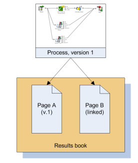
Page A is not linked to the latest version of the process, but Page B is linked. At this point, there is no difference between the behavior of the two pages, because there is only one version of the process.
However, if a new version of the process is created, Page B will reference the new version, because it is always linked to the latest version. Page A, however, will still reference the most recent results from version 1 of the process, because it is not linked:
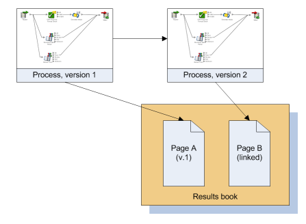
Both options may occasionally result in unexpected behavior in the results book:
-
If a page is linked to the most recent version of a process, but the processor whose data is referenced is deleted from the process, then the results page will become invalid, because there is no data for it to report.
-
If a page is linked to a previous version of a process, and the process is packaged and moved to a new project, there will be no data for the page, and it will be invalid. This is because this instance of the process has not been run in the new context, and so there is no data available for the page to report.
To view a Results Book, select the Results Book in the Project Browser. The pages of the Results Book appear as tabs in the Results Browser.
Sharing a Results Book Externally
The easiest way to share a Results Book externally, for example to send it to a colleague who does not have access to EDQ, is to create a Microsoft Excel workbook containing all of the pages of the Results Book as worksheets. This can be done using the far right icon on the Results Browser.
To create an Excel workbook with just the current page, select Export to Excel.
If you want to write the results in your Results Book out to a file or database on a repeated or regular basis, you can set up a Results Book Export, and schedule it as part of a job. This allows you to automate the output of selected results each time a process, or set of processes, is run. This is useful if you have changing input data and want to store metrics each time the data is analyzed.
To set up a Results Book Export, either right-click on a Results Book and select Export, or right-click on Exports, and select Results Book Export.
1.13 External Tasks
External Tasks are stored details of tasks that are run as part of EDQ Jobs, but which do not occur within the EDQ application.
An External Task may be either a File Download or an External Executable.
File downloads are used to capture files into the server landing area for processing in EDQ. The files may be downloaded from the internet or from other network sources. User authentication details, and proxy/firewall settings where required, can be set as part of the file download task.
The complete set of options that may be set for a File Download task is as follows:
-
URL: specifies the location of the source file - this may be either an internet location or another network file location to which the server can connect. -
Username: specifies a user name, where authentication details are needed to download the file. -
Password: specifies a password, where authentication details are needed to download the file. -
Proxy Host: the name or IP address of the proxy/firewall server, where the server is not directly connected to the internet/network. -
Proxy Port: the port used to connect to the proxy/firewall server. -
Proxy Username: the user name used to authenticate to the proxy/firewall server. -
Proxy Password: the password used to authenticate to the proxy/firewall server. -
Filename: the name to give the downloaded file when it has been downloaded to the landing area. Note that if you want to put the file in a subfolder in the landing area, use forward slashes to specify a directory structure (for example,DownloadedData/downloadedfile.csv). -
Use Project Specific Folder?: ticking this option will automatically put the file into a project-specific landing area. This is normally used where project permissions are in place, so that the landing area can only be accessed by processes within the same project. -
Allow SSL Hostname Mismatch?: ticking this option will allow the download task to ignore discrepancies between the hostname specified in the SSL certificate and the name of the server to which it applies. -
Ignore Invalid SSL Certificate?: ticking this option will allow the download task to ignore unverified SSL certificates on the host.
Finally, you can name the file download task and give it an optional description.
1.13.1 External Executable
The following options may be set for an External Executable task:
-
Command: this option specifies the command that you want to execute. If the path to the command is not on the System Path of the EDQ server, you must specify the full path to the command. -
Arguments: this option specifies any additional arguments you want to provide for the command. -
Working Directory: this option specifies the working directory on the EDQ server where the command will execute. Any files that need to be read by the command must be present in this directory. Also, any files that are written by the command will be written to this directory. Note that if this option is left blank, the working directory for the command will be the server file landing area (which is set to[Install Path]\oedq_local_home\landingareain a default installation).
Finally, you can name the executable task and give it an optional description.
Security Considerations for External Tasks
A property named externaltasks.restricted is used to control the scope of external tasks. This property is set in the director.properties file and is set to true by default.
When externaltasks.restricted is set to true, commands used in external tasks must reside in the EDQ command area. By default, the command area is found at oedq_local_home/commandarea. The location may be overridden by setting the commandarea property in director.properties.
Note that if an external executable needs to run a script, such as a Perl script, the call must be wrapped in a batch file in the command area.
WARNING:
If externaltasks.restricted is set to false, the external executables mechanism represents a potential security hazard. In theory, anyone with access to the Director application could write an external job which has unlimited access to the server, including the ability to delete files, read sensitive data and so on.
1.14 Jobs
A Job is an organized configuration of one or more ordered Tasks. A Task is the execution of a Snapshot, a Process, an Export, a Results Book Export or an External Task.
Jobs are located within Projects.
The Tasks in a Job may be organized into several Phases, which are used to control the order in which Tasks are executed. For example, to ensure a Task A completes before Task B, Task A is placed in one Phase and Task B in a later phase. Within a Phase, all Tasks run as quickly as possible and (wherever possible) in parallel, sharing the available threads. It is possible to run several chained processes in the same Phase, in which case they will effectively run as a single process.
Phases and Tasks can be enabled or disabled, but this can be overridden using a Run Profile when running a job from the Server Console UI, or using the 'runopsjob' command of the EDQ command line interface.
Jobs may also include Triggers, which can be used to stop real-time processes or to start other jobs, either before the other tasks in a phase start running or once they are all complete.
You can configure a Job Notification email to be sent out on completion of a job. The email will show the Job status (that is, whether it succeeded or failed) and will also contain details of any warnings or errors encountered during execution.
Jobs can be scheduled to run using the Director UI, the Server Console UI, or an external scheduler using the Command Line Interface.
Jobs are created and managed using the Job Canvas. To open the Job Canvas, navigate to the Jobs node of a project in the Project Browser and double click it.
The Job Canvas itself is divided into the Phase list (on the left) and the Canvas on the right. The Canvas displays the tasks in the currently selected Phase.
The Project Browser can be hidden (maximizing the area available for the Job Canvas) by toggling the Maximize Jobs Canvas button in the Director toolbar.
The buttons on the Job Canvas tool bar are as follows:
Table 1-130 Job Canvas Toolbar
| Name | Description |
|---|---|
|
Run Job |
Runs the currently displayed Job. |
|
Run Job With Run Profile |
Runs the currently displayed Job after prompting the user to select a Run Profile. |
|
Notification |
Configures an email notification. See Job Notifications for further details. More |
|
Show/Hide Phase List |
Shows/hides the Phase list. |
|
Toggle Tool Palette Item |
If the Filter is activated, the Tool Palette will display only those Tasks that can be connected to the currently selected Task. |
|
Job Externalization |
Opens the Job Externalization dialog for the currently selected Job. |
|
Add Note |
Adds a note to the Job Canvas, which can be moved by clicking and dragging, or deleted by selecting and pressing Delete. |
|
Zoom In and Out |
These buttons are used to zoom in or out on the Job Canvas. |
1.14.1 Creating and Managing Jobs
This topic covers:
Note:
It is not possible to edit or delete a Job that is currently running. Always check the Job status before attempting to change it.Snapshot and Export Tasks in Jobs must use server-side data stores, not client-side data stores.
To create a job:
-
Expand the required project in the Project Browser.
-
Right click the Jobs node of the project and select New Job.
-
The New Job dialog is displayed. Enter a Name and (if required) Description, then click Finish.
-
The Job is created and displayed in the Job Canvas.
-
Right-click New Phase in the Phase list, and select Configure.
-
Enter a name for the phase and select other options as required:
Field Description Enabled?
To enable or disable the Phase. Default state is checked (enabled).
Note: The status of a Phase can be overridden by a Run Profile or with the 'runopsjob' command on the EDQ Command Line Interface.
Execution Condition
To make the execution of the Phase conditional on the success or failure of previous Phases.
The options are:
-
Execute on failure: the phase will only execute if the previous phase did not complete successfully.
-
Execute on success (default): the Phase will only execute if all previous Phases have executed successfully.
-
Execute regardless: the Phase will execute regardless of whether previous Phases have succeeded or failed.
Note: there cannot be an error flag and any existing error flags need to have been removed in a former phase.
Clear Error?
To clear or leave unchanged an error state in the Job.
If a job phase has been in error, an error flag is applied.
Any former error flag must be cleared in the Execute on success phase, in order for an 'Execute on Success' phase to execute.
The default state is unchecked.
Triggers
To configure Triggers to be activated before or after the Phase has run. For more information, see Using Job Triggers. More
-
-
Click OK to save the settings.
-
Click and drag Tasks from the Tool Palette, configuring and linking them as required.
-
To add more Phases, click Add Job Phase button at the bottom of the Phase area. Phase order can be changed by selecting a Phase and moving it up and down the list with the Move Phase buttons. To delete a Phase, click Delete Phase button.
-
When the Job is configured as required, click File > Save.
To edit a job:
-
To edit a Job, locate it within the Project Browser and either double click it or right-click and select Edit....
-
The Job is displayed in the Job Canvas. Edit the Phases and/or Tasks as required.
-
Click File > Save.
Deleting a job does not delete the processes that the Job contained, and nor does it delete any of the results associated with it. However, if any of the processes contained in the Job were last run by the Job, the last set of results for that process will be deleted. This will result in the processors within that process being marked as out of date.
To delete a Job, either:
-
select it in the Project Browser and press the Delete key; or
-
right-click the job and select Delete.
Remember that it is not possible to delete a Job that is currently running.
There are further options available when creating or editing a job, accessible via the right-click menu.
Select a task on the canvas and right click to display the menu. The options are as follows:
-
Enabled - If the selected task is enabled, there will be a checkmark next to this option. Select or deselected as required.
-
Configure Task... - This option displays the Configure Task dialog.
-
Delete - Deletes the selected task.
-
Open - Opens the selected task in the Process Canvas.
-
Cut, Copy, Paste - These options are simply used to cut, copy and paste tasks as required on the Job Canvas.
Editing and Configuring Job Phases
Phases are controlled using a right-click menu. The menu is used to rename, delete, disable, configure, copy and paste Phases.
Use the Add, Delete, Up and Down controls at the bottom of the Phase list.
1.14.2 Using Job Triggers
Job Triggers are used to start or interrupt other Jobs. Two types of trigger are available by default:
-
Run Job Triggers: used to start a Job.
-
Shutdown Web Services Triggers: used to shut down real-time processes.
Further Triggers can be configured by an Administrator, such as sending a JMS message or calling a Web Service. They are configured using the Phase Configuration dialog.
Triggers can be set before or after a Phase. A Before Trigger is indicated by a blue arrow above the Phase name, and an After Trigger is indicated by a red arrow below it.
Triggers can also be specified as Blocking Triggers. A Blocking Trigger prevents the subsequent Trigger or Phase beginning until the task it triggers is complete.
To configure triggers:
-
Right-click the required Phase and select Configure. The Phase Configuration dialog is displayed.
-
In the Triggers area, click the Add Trigger button under the Before Phase or After Phase list as required. The Select Trigger dialog is displayed.
-
Select the Trigger type in the drop-down field.
-
Select the specific Trigger in the list area.
-
Click OK.
-
If required, select the Blocking? checkbox next to the Trigger.
-
Set further Triggers as required.
-
When all the Triggers have been set, click OK.
To delete a trigger from a job:
-
Right-click the required Phase and select Configure.
-
In the Phase Configuration dialog, find the Trigger selected for deletion and click it.
-
Click the Delete Trigger button under the list of the selected Trigger. The Trigger is deleted.
-
Click OK to save changes. However, if a Trigger is deleted in error, click Cancel instead.
1.14.3 Externalizing Jobs
Tasks within Jobs contain a number of settings that can be externalized.
To externalize a setting on a Task:
-
Right-click on the Task and select Configure Task.
-
Click the Externalize button next to the required setting.
-
Select the checkbox in the Externalize pop-up.
-
A default name for the setting is displayed, which can be edited if required.
-
Click OK.
These settings are then managed from the Job Externalization dialog. To open the dialog, click the Job Externalization button on the Job Canvas tool bar.
Externalization for a Job can be enabled or disabled by checking or clearing the Enable Externalization box.
The Externalized Options area shows the options that are available for externalization.
To delete an option, select it and click Delete (under the Externalized Options area).
To rename an option, select it and click Rename. Edit the name in the Rename pop-up and click OK.
The Externalized Tasks area shows the selected option next to the Task it is associated with. If an option is associated with more than Task, it is listed once for each Task. The example dialog above shows that the Enabled option is associated with the UK Customers and US Customers tasks.
To disassociate an option from a Task, select it in this area and click Delete.
1.14.4 Execution Options
EDQ can execute the following types of task, either interactively from the GUI (by right-clicking on an object in the Project Browser, and selecting Run), or as part of a scheduled Job.
The tasks have different execution options. Click on the task below for more information:
-
External Tasks (such as File Downloads, or External Executables)
-
Exports (of data)
In addition, when setting up a Job it is possible to set Triggers to run before or after Phase execution.
When setting up a Job, tasks may be divided into several Phases in order to control the order of processing, and to use conditional execution if you want to vary the execution of a job according to the success or failure of tasks within it.
When a Snapshot is configured to run as part of a job, there is a single Enabled? option, which is set by default.
Disabling the option allows you to retain a job definition but to disable the refresh of the snapshot temporarily - for example because the snapshot has already been run and you want to re-run later tasks in the job only.
There are a variety of different options available when running a process, either as part of a job, or using the Quick Run option and the Process Execution Preferences:
-
Readers (options for which records to process)
-
Process (options for how the process will write its results)
-
Run Modes (options for real time processes)
-
Writers (options for how to write records from the process)
For each Reader in a process, the following option is available:
Sample?
The Sample option allows you to specify job-specific sampling options. For example, you might have a process that normally runs on millions of records, but you might want to set up a specific job where it will only process some specific records that you want to check, such as for testing purposes.
Specify the required sampling using the option under Sampling, and enable it using the Sample option.
The sampling options available will depend on how the Reader is connected.
For Readers that are connected to real time providers, you can limit the process so that it will finish after a specified number of records using the Count option, or you can run the process for a limited period of time using the Duration option. For example, you can run a real time monitoring process for a period of 1 hour only.
For Readers that are connected to staged data configurations, you can limit the process so that it runs only on a sample of the defined record set, using the same sampling and filtering options that are available when configuring a Snapshot. For example, you can run a process so that it only processes the first 1000 records from a data source.
The Sampling Options fields are as follows:
-
All - Sample all records.
-
Count - Sample n records. This will either be the first n records or last n records, depending on the Sampling Order selected.
-
Percentage - Sample n% of the total number of records.
-
Sampling Offset - The number of records after which the sampling should be performed.
-
Sampling Order - Descending (from first record) or Ascending (from last).
Note:
If a Sampling Offset of, for example, 1800 is specified for a record set of 2000, only 200 records can be sampled regardless of the values specified in the Count or Percentage fields.The following options are available when running a process, either as part of the Process Execution Preferences, or when running the process as part of a job.
| Option | Description |
|---|---|
|
Use Intelligent Execution? |
Intelligent Execution means that any processors in the process which have up-to-date results based on the current configuration of the process will not re-generate their results. Processors that do not have up-to-date results are marked with the rerun marker. Intelligent Execution is selected by default. Note that if you choose to sample or filter records in the Reader in a process, all processors will re-execute regardless of the Intelligent Execution setting, as the process will be running on a different set of records. |
|
Enable Sort/Filter in Match processors? |
This option means that the specified Sort/Filter enablement settings on any match processors in the process (accessed via the Advanced Options on each match processor) will be performed as part of the process execution. The option is selected by default. When matching large volumes of data, running the Sort/Filter enablement task to allow match results to be reviewed may take a long time, so you may want to defer it by de-selecting this option. For example, if you are exporting matching results externally, you may want to begin exporting the data as soon as the matching process is finished, rather than waiting until the Enable Sort/Filter process has run. You may even want to over-ride the setting altogether if you know that the results of the matching process will not need to be reviewed. |
|
Results Drill Down |
This option allows you to choose the level of Results Drill Down that you require.
|
|
Publish to Dashboard? |
This option sets whether or not to publish results to the Dashboard. Note that in order to publish results, you first have to enable dashboard publication on one or more audit processors in the process. |
To support the required Execution Types, EDQ provides three different run modes.
If a process has no readers that are connected to real time providers, it always runs in Normal mode (see below).
If a process has at least one reader that is connected to a real time provider, the mode of execution for a process can be selected from one of the following three options:
In Normal mode, a process runs to completion on a batch of records. The batch of records is defined by the Reader configuration, and any further sampling options that have been set in the process execution preferences or job options.
Prepare mode is required when a process needs to provide a real time response, but can only do so where the non real time parts of the process have already run; that is, the process has been prepared.
Prepare mode is most commonly used in real time reference matching. In this case, the same process will be scheduled to run in different modes in different jobs - the first job will prepare the process for real time response execution by running all the non real time parts of the process, such as creating all the cluster keys on the reference data to be matched against. The second job will run the process as a real time response process (probably in Interval mode).
In Interval mode, a process may run for a long period of time, (or even continuously), but will write results from processing in a number of intervals. An interval is completed, and a new one started, when either a record or time threshold is reached. If both a record and a time threshold are specified, then a new interval will be started when either of the thresholds is reached.
As Interval mode processes may run for long periods of time, it is important to be able to configure how many intervals of results to keep. This can be defined either by the number of intervals, or by a period of time.
For example, you can set options for a real time response process that runs on a continuous basis, starting a new interval every day. For example, you could retain a maximum of 10 intervals (or 10 days of results).
Note that processes that run continuously may also publish their results to the Dashboard, so that trend analysis can be plotted across time and record intervals.
Browsing Results from processing in Interval mode
When a process is running in Interval mode, you can browse the results of the completed intervals (as long as they are not too old according to the specified options for which intervals to keep).
The Results Browser presents a simple drop-down selection box showing the start and end date and time of each interval. By default, the last completed interval is shown. Select the interval, and browse results.
If you have the process open when a new set of results becomes available, you will be notified in the status bar. You can then select these new results using the drop-down selection box.
For each Writer in a process, the following options are available:
-
Write Data?This option sets whether or not the writer will 'run'; that is, for writers that write to stage data, de-selecting the option will mean that no staged data will be written, and for writers that write to real time consumers, de-selecting the option will mean that no real time response will be written.This is useful in two cases:
1. You want to stream data directly to an export target, rather than stage the written data in the repository, so the writer is used only to select the attributes to write. In this case, you should de-select the Write Data option and add your export task to the job definition after the process.
2. You want to disable the writer temporarily, for example, if you are switching a process from real time execution to batch execution for testing purposes, you might temporarily disable the writer that issues the real time response.
-
Enable Sort/Filter?This option sets whether or not to enable sorting and filtering of the data written out by a Staged Data writer. Typically, the staged data written by a writer will only require sorting and filtering to be enabled if it is to be read in by another process where users might want to sort and filter the results, or if you want to be able to sort and filter the results of the writer itself.The option has no effect on writers that are connected to real time consumers.
Any External Tasks (File Downloads, or External Executables) that are configured in a project can be added to a Job in the same project.
When an External Task is configured to run as part of a job, there is a single Enabled? option.
Enabling or Disabling the Enable export option allows you to retain a job definition but to enable or disable the export of data temporarily.
When an Export is configured to run as part of a job, the export may be enabled or disabled (allowing you to retain a Job definition but to enable or disable the export of data temporarily), and you can specify how you want to write data to the target Data Store, from the following options:
Delete current data and insert (default)
EDQ deletes all the current data in the target table or file and inserts the in-scope data in the export. For example, if it is writing to an external database it will truncate the table and insert the data, or if it is writing to a file it will recreate the file.
Append to current data
EDQ does not delete any data from the target table or file, but adds the in-scope data in the export. When appending to a UTF-16 file, use the UTF-16LE or UTF-16-BE character set to prevent a byte order marker from being written at the start of the new data.
Replace records using primary key
EDQ deletes any records in the target table that also exist in the in-scope data for the export (determined by matching primary keys) and then inserts the in-scope data.
Note:
When an Export is run as a standalone task in Director (by right-clicking on the Export and selecting Run), it always runs in Delete current data and insert mode.Delete current data and insert and Replace records using primary key modes perform Delete then Insert operations, not Update. It is possible that referential integrity rules in the target database will prevent the deletion of the records, therefore causing the Export task to fail. Therefore, in order to perform an Update operation instead, Oracle recommends the use of a dedicated data integration product, such as Oracle Data Integrator.
When a Results Book Export is configured to run as part of a job, there is a single option to enable or disable the export, allowing you to retain the same configuration but temporarily disable the export if required.
Triggers are specific configured actions that EDQ can take at certain points in processing.
Before Phase execution in a Job
After Phase execution in a Job
When making manual match decisions (for example to notify another application when a decision is made that affects that application, such as whether or not an individual is a genuine match against a watchlist).
1.14.5 Job Notifications
A Job may be configured to send a notification email to a user, a number of specific users, or a whole group of users, each time the Job completes execution. This allows EDQ users to monitor the status of scheduled jobs without having to log on to EDQ.
Emails will also only be sent if valid SMTP server details have been specified in the mail.properties file in the notification/smtp subfolder of the oedq_local_home directory. The same SMTP server details are also used for Issue notifications.
The default notification template - default.txt - is found in the EDQ config/notification/jobs directory. To configure additional templates, copy this file and paste it into the same directory, renaming it and modifying the content as required. The name of the new file will appear in the Notification template field of the Email Notification Configuration dialog.
Configuring a Job Notification
To configure a job notification:
-
Open the Job and click Configure Notification button on the Job Canvas toolbar. The Email Notification Configuration dialog is displayed.
-
Check the Enabled? box.
-
Select the Notification template from the drop-down list.
-
Click to select the Users and Groups to send the notification to. To select more than one User and/or Group, hold down the CTRL key when clicking.
-
Click OK.
Note:
Only users with valid email addresses configured in User Configuration will receive emails.The default notification contains summary information of all tasks performed in each phase of a job, as follows:
The notification displays the status of the snapshot task in the execution of the job. The possible statuses are:
-
STREAMED - the snapshot was optimized for performance by running the data directly into a process and staging as the process ran
-
FINISHED - the snapshot ran to completion as an independent task
-
CANCELLED - the job was canceled by a user during the snapshot task
-
WARNING - the snapshot ran to completion but one or more warnings were generated (for example, the snapshot had to truncate data from the data source)
-
ERROR - the snapshot failed to complete due to an error
Where a snapshot task has a FINISHED status, the number of records snapshotted is displayed.
Details of any warnings and errors encountered during processing are included.
The notification displays the status of the process task in the execution of the job. The possible statuses are:
-
FINISHED - the process ran to completion
-
CANCELLED - the job was canceled by a user during the process task
-
WARNING - the process ran to completion but one or more warnings were generated
-
ERROR - the process failed to complete due to an error
Record counts are included for each Reader and Writer in a process task as a check that the process ran with the correct number of records. Details of any warnings and errors encountered during processing are included. Note that this may include warnings or errors generated by a Generate Warning processor.
The notification displays the status of the export task in the execution of the job. The possible statuses are:
-
STREAMED - the export was optimized for performance by running the data directly out of a process and writing it to the data target
-
FINISHED - the export ran to completion as an independent task
-
CANCELLED - the job was canceled by a user during the export task
-
ERROR - the export failed to complete due to an error
Where an export task has a FINISHED status, the number of records exported is displayed.
Details of any errors encountered during processing are included.
The notification displays the status of the results book export task in the execution of the job. The possible statuses are:
-
FINISHED - the results book export ran to completion
-
CANCELLED - the job was canceled by a user during the results book export task
-
ERROR - the results book export failed to complete due to an error
Details of any errors encountered during processing are included
The notification displays the status of the external task in the execution of the job. The possible statuses are:
-
FINISHED - the external task ran to completion
-
CANCELLED - the job was canceled by a user during the external task
-
ERROR - the external task failed to complete due to an error
Details of any errors encountered during processing are included
1.14.6 Command-Line Interface
A collection of command line utilities are provided with EDQ in the file jmxtools.jar.
The commands in jmxtools.jar can be used from the location where EDQ is installed. The command syntax is as follows:
java.exe -jar jmxtools.jar <command> <arguments> <argument options>
Each command can take a range of different arguments, which are case sensitive.
Commands, arguments and options
This section lists all of the commands available using the Command Line tool, and any arguments used by each command.
The droporphans command is used to remove any orphaned results tables.
The droporphans command takes several additional arguments as follows:
The listorphans command is used to identify any orphaned results tables. See the Identifying and removing orphaned tables section of the EDQ Server Administration Guide for further information. The listorphans command takes the same arguments as the droporphans command above.
The scriptorphans command creates a list of SQL commands for dropping orphaned results tables. This is useful if you wish to review exactly which commands will run on the Results database when you drop tables, or if you wish to drop the tables yourself manually.
The list command lists all the available commands.
The runjob command runs a named job in the same way as if running the job using the Director UI. The runjob command takes several additional arguments as follows:
The runopsjob command runs a named job in the same way as if running the job using the Server Console UI. This provides additional functionality to the runjob command - specifically the use of Run Labels and Run Profiles. Run Labels may be used to store results separately from other runs of the same job. Run Profiles may be used to override externalized configuration settings at runtime.
The runopsjob command takes several additional arguments as follows:
The shutdown command shuts down all real-time jobs; that is jobs that are running from real-time record providers (web services or JMS).
This takes several additional arguments as follows:
The following example command runs a job from the command line interface:
java.exe -jar jmxtools.jar runjob -job Job1 -project ClientProject -u adminuser -p adminpassword server:9005
This command specifies that:
-
the job is called 'Job1'
-
the project is called 'ClientProject'
-
the user is 'adminuser'
-
the password is 'adminpassword',
-
the server name is 'server'
-
and the port for the command line interface is 9005.
Note:
Any names (such as project or user names) that contain spaces must be encased in double quotes in the command syntax. For example, if the project containing the job that you want to call is named 'Master Data Analysis' the command must use the syntax '...-project "Master Data Analysis"...'When a job is completed, an exit status (0 or 1) is returned. An exit status of 0 indicates the job completed successfully, and an exit status of 1 indicates that there was a failure in the Job.
The following example syntax for a Windows batch file shows a simple way of calling a named job in EDQ, and using the returned exit status to display an error message where the job failed:
@ECHO OFF
java -jar jmxtools.jar runjob -job [Job Name] -project [Project Name] -u [User Name] -p [Password] [Server Name]:9005
IF ERRORLEVEL 1 GOTO error
ECHO Job ran successfully
GOTO end
:error
ECHO An error occurred running the job
:end
1.15 Exports
There are two types of Export:
-
A prepared export (Staged Data Export or Results Book Export) which uses a saved configuration.
-
An ad-hoc export of the current results from the Results Browser to an Excel file.
A Prepared Export is a saved configuration for outputting Staged Data or Results Books to a Data Store, either to a table in a database, or to a file.
A Staged Data Export can map Staged Data attributes to the attributes in an external database table or file, or it can auto-create the target database table or file when it runs. You can define whether data should be appended to the table, whether the data should be overwritten, or whether to replace only target records with a matching primary key in the staged data set.
Exports are defined separately from Writers in processes to allow more flexibility. For example, it is possible to export the same set of Staged Data to different targets, and to use a different set of attribute names in EDQ to those used in an external database or file.
A Results Book Export can either auto-create the target database table or file when it runs, or replace an existing table or file with the same name. Where the table or file already exists the data will be overwritten.
A Prepared Export can be run in two ways:
-
Manually. That is, you have some Staged Data or a saved Results Book and you want to write it externally. To run an export manually, right-click on the Export in the Project Browser, and select Run Export.
-
Automatically. That is, you want to export data as part of a scheduled job. To run an export as part of a scheduled job, define a job, and add the Export as a task, and then use the Scheduler to schedule the job.
Note:
Data does not need to be staged in the EDQ repository when running a staged data export as part of a job. If you include the export task within your job, but disable the staged data in the job definition, the output data will be 'streamed' directly into the Export target.The Ad-hoc export enables a one-off export of data in the Results Browser to an Excel file. The export may be of a selection of data, or where no data is selected, the export will be of all the results viewable in the current Results Browser tab.
Export all tabs to Excel enables an ad-hoc export of all tabs in the Results Browser. Each Results Browser tab will be written to a worksheet in the Excel file.
The ad-hoc export is subject to user-definable preferences (Edit menu, Preferences) to define:
-
The maximum number of rows that are exportable
-
Whether to export the Result Browser column names as a header
-
Whether to open the Excel file after writing to the file.
1.16 Notes
Director allows users to capture notes throughout the progress of a project. The use of notes allows you to use Director as the definitive repository for all information associated with the project. Any information that needs to be made available to all users working on a project can be added as a note.
You may store the following information in each Note:
-
A title
-
A free-text note
-
Optional file attachments
The user and date/time of note creation are automatically captured, as are the user and date/time of the last modification made to the note.
The following are examples of the use of notes:
-
Giving brief contact details of the main project sponsor
-
Attaching a project plan
-
Attaching a project definition document
-
Attaching a spreadsheet dividing up assigned work amongst several users
-
Attaching an email thread with the initial discussion of the project
Note:
The maximum size for each attachment is 2MB.Attachments are imported into the database. If you want to store attachments in a common network directory in order to ensure that the latest version is always used, you might simply add a Project Note to inform users where to access all the documents related to the project.
1.17 Web Services
EDQ processes as configured in Director can be deployed as Web Services to provide easy integration with source systems for real time data auditing, cleansing and matching (for example, for real time duplicate prevention).
This allows you to ensure that data problems are prevented at the point of data entry by using an integrated data quality Web Service to check records as they are entered.
Right-click on Web Services in the Project Browser, and select New Web Service.
Use the wizard to define the inbound and outbound interfaces of your Web Service. Once these interfaces are defined, you can then change a process to act as a Web Service by configuring the Reader to read from a real time provider (the inbound interface), and configuring the Writer to write to a real time consumer (the outbound interface). Note that the outbound interface is optional - for example, for Real time monitoring processes that check records as they are entered but do not issue responses.
For some Web Services, it is useful to consider multiple records as part of the same message. For example, when setting up a Web Service to match records in real time, in order to prevent duplicate records from being entered into systems, both the inbound and outbound interfaces of the Web Service should have the Multi-record? option ticked, so that a single message can be received with all candidate records, and a single message can be sent with the possible duplicate records and their match levels.
You can also set the Multi-record option differently on the inbound and outbound interfaces. For example, if matching a single inbound record against Reference Data sets managed by EDQ (such as when checking customer records against watchlists), the inbound interface may be single record, but the outbound interface may be multi-record, as the input record may match several lists.
To copy the URL of the WSDL file for a Web Service, right-click on it, and select Copy WSDL URL to clipboard.
All the Web Services that are set up on an EDQ server can be viewed from a single page so that integrators can easily access the WSDL files required to use them.
To see all the Web Services on a server:
-
Go to the EDQ Launchpad.
-
Click on Web Services.
-
Log on with your normal user name and password.
From this page, you can see the Service URLs of the Web Services, view the generated WSDL files for its available operations (provider and consumer), and (if the service is running) test the Web Service using an automatically generated GUI.
The (test) option launches a separate Java application for testing the Web Services on a server. This includes an option to test the response time of the Web Service.
Note:
If you are a user with restricted project access, you will only see, and will only be able to test, the Web Services for the projects to which you have access.Setting up the Process for a Web Service
Once a Web Service has been defined, you can configure the Reader of a process to read messages from its inbound interface (real time provider), and (optionally) you can configure the Writer of a process to issue a response by connecting it to the outbound interface (real time consumer).
To switch easily between Batch and Real time processing (for example to switch to Batch mode in order to test a process), it is useful to configure the process to read its data from a Data Interface, and use Data Interface Mappings to switch between a Staged Data source (such as a snapshot) and a Real time provider (such as a Web Service).
Another useful mechanism when designing a real time process, and switching between Batch and Real time execution in order to test it, is to add two writers to the process - one issuing the real time response, and one writing an audit trail of both the inbound record and the response to a staged data table. You can then configure two different Jobs - one job with the real time writer enabled and the staged data writer disabled, and another job with the staged data writer enabled and the real time writer disabled. See Execution Options for more information. More
The process linked to a Web Service will be either a Real time response process (accepting inbound messages and issuing a real time response), or a Real time monitoring process (checking records as they are added but not issuing a response). As the process is likely to run continuously, it is advisable to run it in Interval mode so that it writes results on a periodic basis.
A Java application is accessible from the EDQ Launchpad that allows you to test a running Web Service before any integration work is done. To access the application, click on the (test) option when viewing the Web Services from the Launchpad. You will need to log in again using a valid EDQ user name and password.
The Web Service you selected on the Launchpad will be selected by default, though you can select different services to test using the Project and Web Service drop downs in the Setup section at the top.
The Get WSDL button retrieves the latest WSDL file, if the Web Service has been changed. This allows you to edit the Web Service definition without having to leave the test application.
The remainder of the screen shows In and Out sections. Here you can set up a request, send it to a Web Service, and see the response.
Note that the Response time of the service to respond to the request is measured in milliseconds.
If required, you can send the request many times and chart the average timings of the responses. To do this, click on the Timing test... button and enter the number of times you want to send the request, and (if required) an interval in milliseconds between sending each request. Then click Run to send the requests. The Status section updates as the requests are sent.
You can then click on the Chart link to generate a chart showing a chart of the responses, so that you can see when the slowest and fastest responses happened:
For a Web Service that expects multiple records - that is, the Web Service was created with the Multi Record? option ticked (for example, a Web Service to identify matching records from a set of candidates) - you can use the Add Record button to add as many records as you require before sending the request. The Add Record button is disabled when a Web Service that expects a single record is selected.
Alternative Integration Methods (JMS)
EDQ also supports integration with its real time capabilities via JMS (Java Messaging Service). In this case, the real time providers and consumers must be set up manually.
1.18 Issues
The use of issues allows users of EDQ to keep a record of their key findings when analyzing data, and also provides a way for work on a project to be allocated and tracked amongst several users.
A typical use of issues might be to capture pieces of intelligence discovered when conducting an audit of data, and to collate a list of actions that require completion - for example, ways in which data quality issues need to be resolved by cleansing.
Amongst other purposes, this allows different users of EDQ to specialize in different activities. For example, audit users can analyze data and pass on information and outstanding issues to specialist data cleansing users.
Issues assigned to the currently logged on user are indicated in the Director Toolbar.
Clicking this notification will open the Issue Manager application. See Issue Manager for further information.
Issues are created from results in the Results Browser, and by the assignment of match results for review. For example, to create an issue based on the Quickstats Profiler's results for the Postcode attribute, right-click on the result and select Create Issue.
This brings up the Issue Creation dialog. The issue is automatically linked with the processor that you created the issue from. If you then assign the issue to another user, that user will be able to link through directly to the relevant processor's results.
Using Issues when Reviewing Matching Results [Match Review only]
Issues are also used when assigning match results for review in the Match Review application. In this case, the user assigning the results for review creates an issue and assigns it to either a specific user, or to a group of users. The issue includes a URL that can be used to open a standalone reviewing application, so that reviewing users do not have any access to the configuration of the processes used to generate the results.
See Using Match Review for more information. More
An administrator can configure EDQ such that users receive an email when issues that are relevant to them are created or changed.
To do this, the administrator must set up valid SMTP server details in the mail.properties file in the notification/smtp subfolder of oedq_local_home directory. The same SMTP server details are also used for Job notifications. See the EDQ Server Administration Guide.
A default template defining the layout and content of the issue email notification is provided. This can be changed if required.
The emails contain a link to open the issue. For issues raised from results the link will open the EDQ Issue Manager, and for issues assigned in order to review match results, this will open the Match Review application with the relevant results selected.
If issue emails are enabled, users with email addresses set up in EDQ (in the User Configuration pages) will receive emails as shown in the below table. Note that if many of these events occur in a single action (for example, if an issue is created by and assigned to the same user), only a single email is sent:
1.19 Snapshots
A snapshot is a staged copy of data in a Data Store that is used in one or more processes.
Note that you do not have to copy the data that you are working with, but doing so allows you greater access to Director's results browsing functionality, as you are able to drill down on processor metrics to see the data itself, at each stage in your processing.
Commonly, you might take a copy of the data when working on an audit process, or when defining the rules for data cleansing, but you might run a process in streaming mode (that is, without copying data into the repository) when you run a data cleansing process in production, in order to save time in execution.
You may define the following properties of a snapshot:
-
The Data Store of the source data (from a list of connected data stores registered on the EDQ host)
-
The table or Data Interface to snapshot (or you may specify SQL to snapshot a new Data Interface)
-
The columns that you want to include in the snapshot
-
Whether or not you want to enable sort and filtering on the snapshot, and on which columns. See Enabling sorting and filtering on snapshots for more details.
-
Basic filter options on the snapshot (or you may write your own SQL WHERE clause for snapshots from database tables)
-
Optional sampling of the data (for example, the first n records, the first n records after an offset, or 1 record in every 100)
-
Optional No Data Handling
Once a snapshot configuration has been added, you can run the snapshot by right-clicking on it in the Project Browser, and selecting Run Snapshot.
Alternatively, you may choose to run the snapshot when you run the first process that uses it.
Snapshots are shared at the project level. This means that many processes in the same project may use the same snapshot, but processes in different projects may not. If you copy and paste a Snapshot configuration into a new project, this is an independent snapshot, and you will need to run it in order to use the staged data in a process (unless you are streaming data from the data source).
You can edit a snapshot using a Right-click menu option - for example to change the size of sample that you are working from.
If you choose to rename a snapshot, and that snapshot is used in processes, those processes will be invalidated. They will not automatically point at the renamed snapshot. Processes refer to snapshots by name so that you can easily move configurations between servers, where internal IDs would be different.
If required, you can also delete a snapshot using a Right-click menu option. Note that if the snapshot is used by other configuration objects, a warning will be displayed as these objects may be in error.
It is normally best to snapshot all columns, and select those you want to work with in a given process by configuring the Reader.
It is possible to normalize various forms of No Data when data is copied into the repository as part of a snapshot. To do this, a Reference Data map is specified that lists a number of characters that are considered as No Data. Typically, these characters will be non-printing characters, such as ASCII characters 0-32. Whenever a data value consists only of No Data characters, it is normalized to a single value. In the default No Data Handling Reference Data, all No Data values are normalized to NULL values. This allows you to distinguish clearly between data that has some kind of value in it, and data that does not.
There are two types of snapshot:
-
Server-side snapshots (that is, snapshots from server-based data stores);
-
Client-side snapshots (that is, snapshots from client-based data stores).
Server-side snapshots are used where the EDQ host server has access to the data that needs to be copied - for example, it is either on the same machine, or on another machine to which the host has a local network connection.
Server-side snapshots may be reloaded either manually or automatically (for example, as part of a scheduled job) whenever the server has access to the data source. This means that when a process is scheduled for execution, it can automatically rerun the snapshot and pick up any changes in the data if required.
Client-side snapshots are used for sources of data that are accessed via the client rather than the server. For example, the data you want to work with might be stored on a client machine that does not have a EDQ host installed (that is, the client accesses an EDQ host on the network). In this case, the data is copied to the EDQ host's repository via connectors on the client.
Client-side snapshots may only be reloaded manually, by a user on a connected client machine with access to the data source - that is, by right-clicking on the snapshot, and selecting Run.
You can cancel the running of a snapshot via a right click option. Once canceled, the snapshot icon in the Project Browser tree is overlaid with the canceled indicator. If the snapshot is subsequently rerun successfully the canceled indicator is removed.